Table of Contents 
Introduction
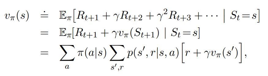
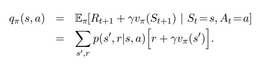
Iterative Policy Evaluation Methods
Iterative Control Methods
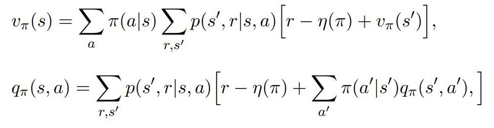
Average Reward Setting
Introduction 
Introduction
Reinforcement learning can be used to solve large problems, e.g.
- Backgammon: $10^{20}$ states
- Computer Go: $10^{170}$ states
- Helicopter: continuous state space
How can we use the methods learnt previously on such huge state-spaces?
For eg: A Tabular methods using only Value Function of states (In half Precision) for the game of Backgammon:
- Memory Requirement: $\frac{10^{20} \times 2}{10^{15}} = $2 Lac PetaBytes
Story so far...
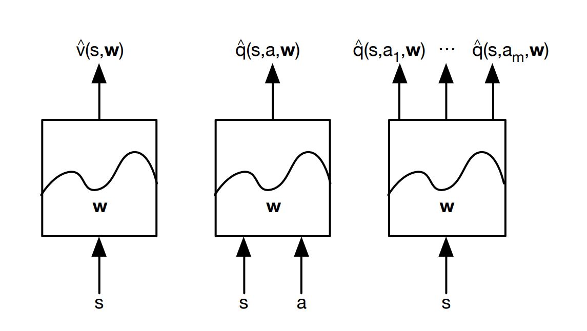
- So far we have represented value function by a lookup table;
- Every state $s$ has an entry $V(s)$
Or every state-action pair $s,a$ has an entry $Q(s, a)$.
- Problem with large MDPs:
- There are too many states and/or actions to store in memory
- It is too slow to learn the value of each state individually
- Solution for large MDPs:
- Estimate value function with function approximation
### $$\hat{v}(s, w) \sim v_\pi(s)$$
or
### $$\hat{q}(s, a, w) \sim q_\pi(s, a)$$
- Estimate value function with function approximation
Generalise from seen states to unseen states;
Update parameter w using MC or TD learning
- Many statistical methods assume a static training set over which multiple passes are made.
- Our situation:data is aquired Online.
- Essential to learn efficiently from incrementally acquired data.
- Reinforcement learning generally requires approximation methods able to handle nonstationary target functions
- In General Control Mechanism, we often seek to learn $q_\pi$ while $\pi$ changes.
- Bootstrapping methods: The target values of training examples are nonstationary
- Methods that cannot easily handle such nonstationarity are less suitable for reinforcement learning.
Incremental Methods 
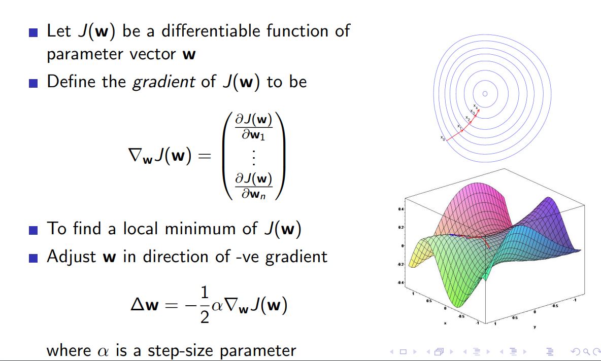
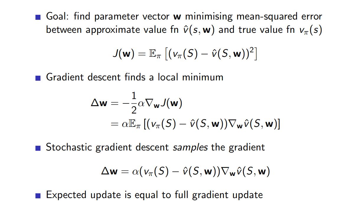
Gradient Descent
The Prediction Objective (MSVE)
- Mean Squared Value Error, or MSVE: ### $$ MSVE(\theta) = \sum_{s \in S}^{}{d(s) \big[ v_\pi (s)-\hat(v)(s,\theta) \big]^2}$$
- Weighting or distribution $d(s) \ge 0$ representing how much we care about the error in each state $s$.
- Why was $d(s)$ not required in Tabular methods?
- because the learned value function could come to equal the true value function exactly.
- learned values at each state were decoupled—an update at one state affected no other.
- More states than weights
- making one state’s estimate more accurate leads to making others’ less accurate.
- We must specify which states we care most about.
Our ultimate purpose is to use it in finding a better policy.
- The best value function for this purpose is not necessarily the best for minimizing MSVE.
Generally,if not specified, consider $d(s) = 1, \forall s \in S $
Stochastic Gradient Descent for MSVE 
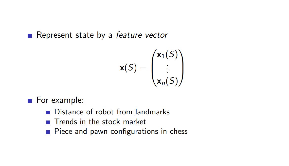
Feature Vector 
Linear Value Function Approximation 
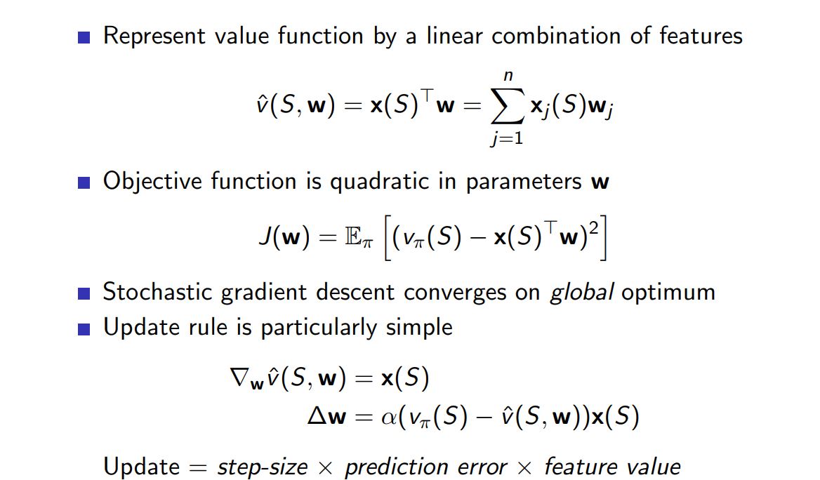
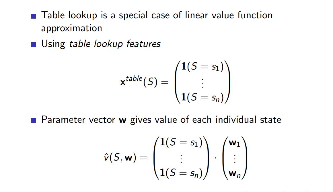
Table Look-up 
Incremental Prediction Methods 
Incremental Prediction Methods 
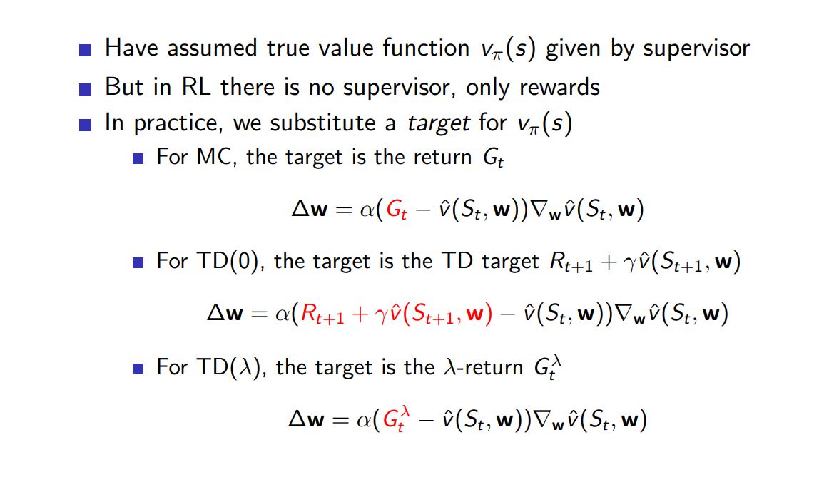
Important Point.
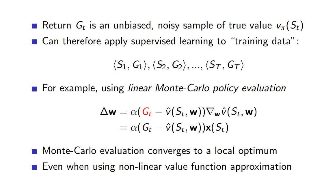
- The Monte Carlo target $U_t = G_t$ is by definition an unbiased estimate of $v_\pi(S_t)$.
- In this situation, SGD method converges to a locally optimal approximation to $v_\pi(S_t)$.
- Bootstrapping targets such as $n$-step returns $G^{(n)}_{t}$ or the DP target, all depend on the current value of the weight vector $\theta_t$.
- Implies that they will be biased
- will not produce a true gradient-descent method
- we call them semi-gradient methods.
- Disadvantage:semi-gradient (bootstrapping) methods do not converge as robustly as gradient methods.
- they do converge reliably in cases such as the linear approximation.
- Advantage:
- Typically significantly faster to learn
- Enable learning to be continual and online
- provides computational advantages.
Monte-Carlo with Value Function Approximation 
TD Learning with Value Function Approximation 
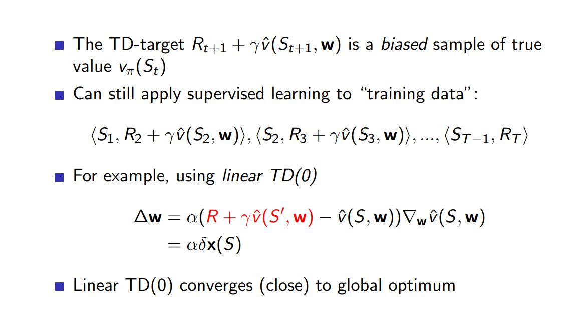
TD($\lambda$) with Value Function Approximation 
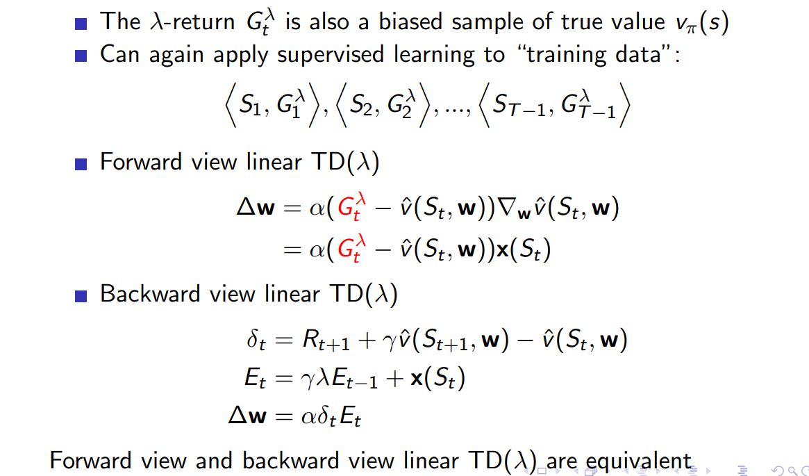
TD($\lambda$) with Value Function Approximation 
- TD converges to a point called the TD-fixedpoint(see references)
$$MSVE(\theta_{TD}) \le \frac{1}{1-\gamma} min_\theta(MSVE(\theta))$$
- $\gamma$ is often near one
- the expansion factor can be quite large,
- there can be substantial loss in asymptotic performance with the TD method.
- However, recall that the TD methods often
- have vastly reduced variance compared to Monte Carlo methods, and
- are faster.
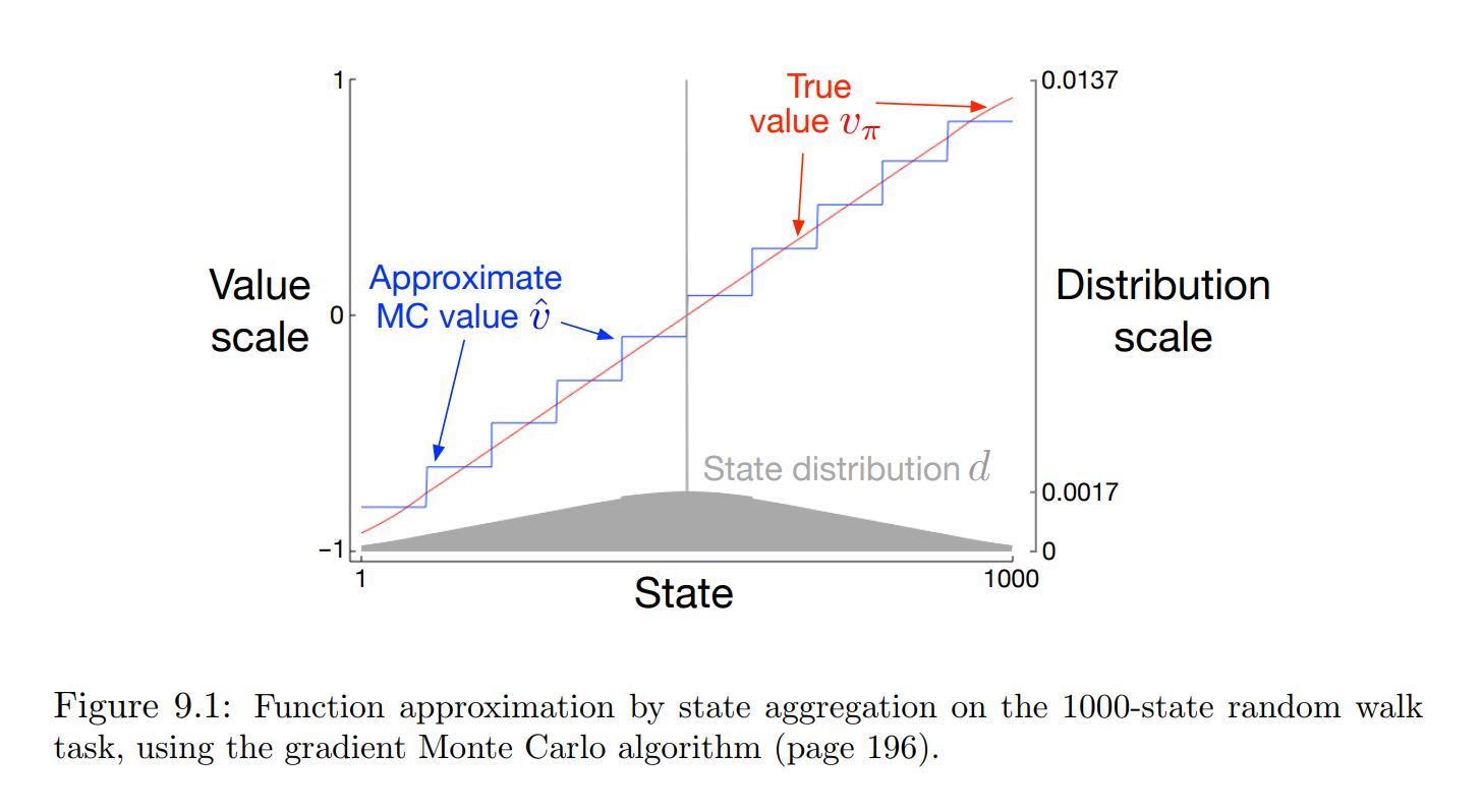
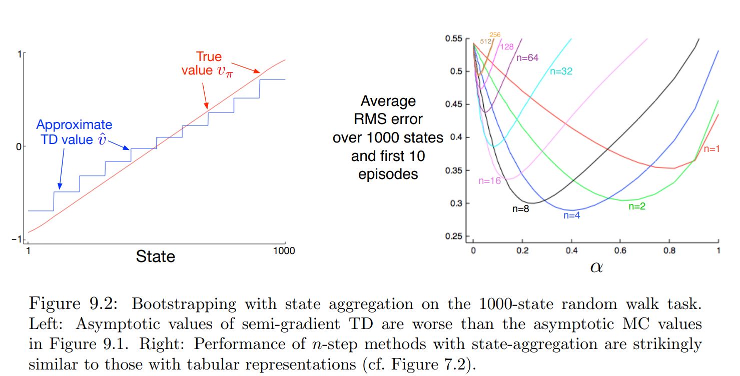
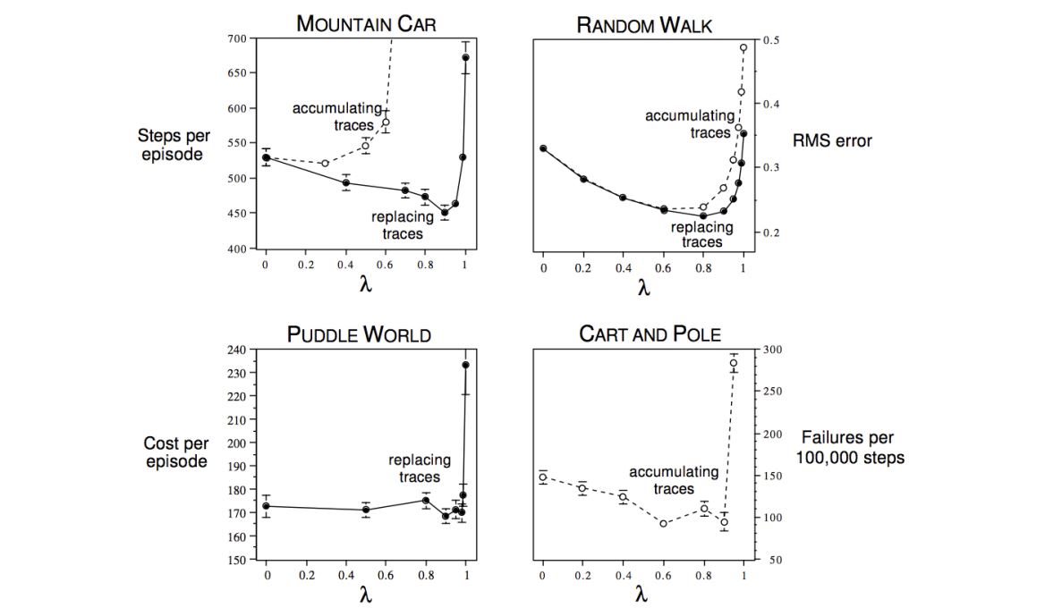
State Aggregation on the 1000-state Random Walk 
A simple form of generalizing function approximation in which states are grouped together.
One estimated value (one component of the weight vector $\theta$) for each group.
Problem Statement
- A 1000-state version of the random walk task
- States are numbered from 1 to 1000, left to right,
- all episodes begin near the center, in state 500
- State transitions are from the current state to one of the 100 neighboring states to its left or right
- With equal probability
- Termination on the left produces a reward of −1, and termination on the right produces a reward of +1.
- All other transitions have a reward of zero
Iterative Control Approximation 
Control with Value Function Approximation 
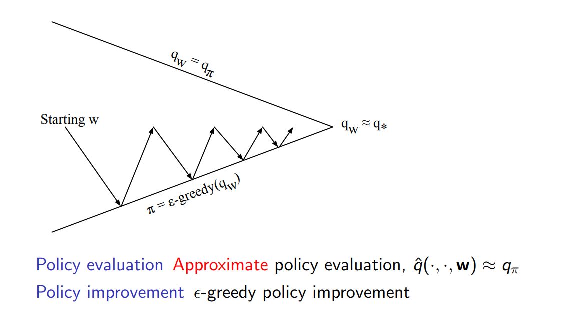
Action-Value Function Approximation 
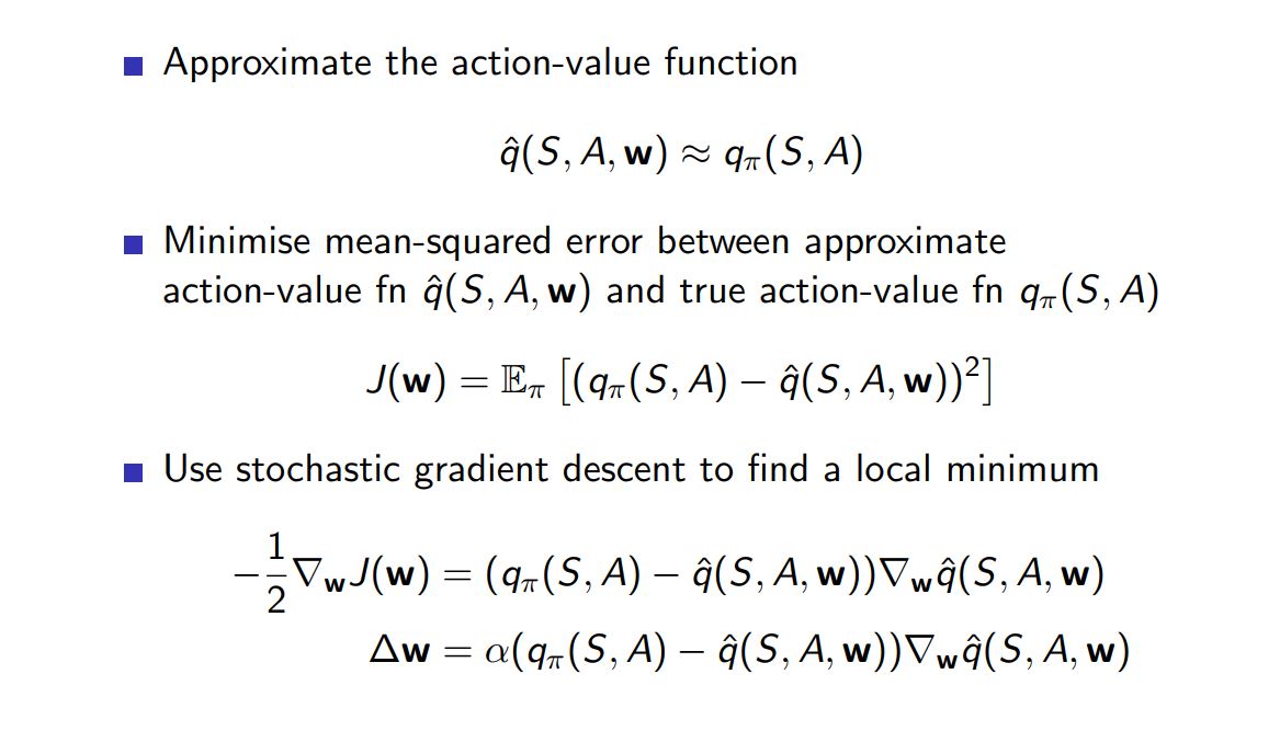
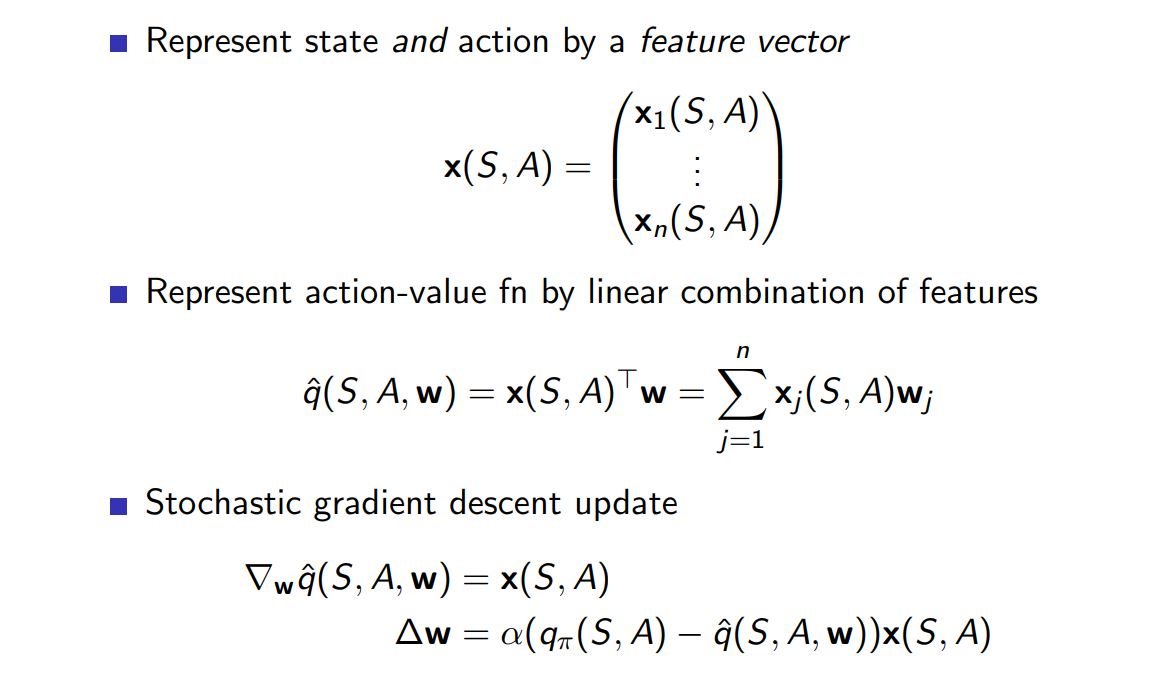
Linear Action-Value Function Approximation 
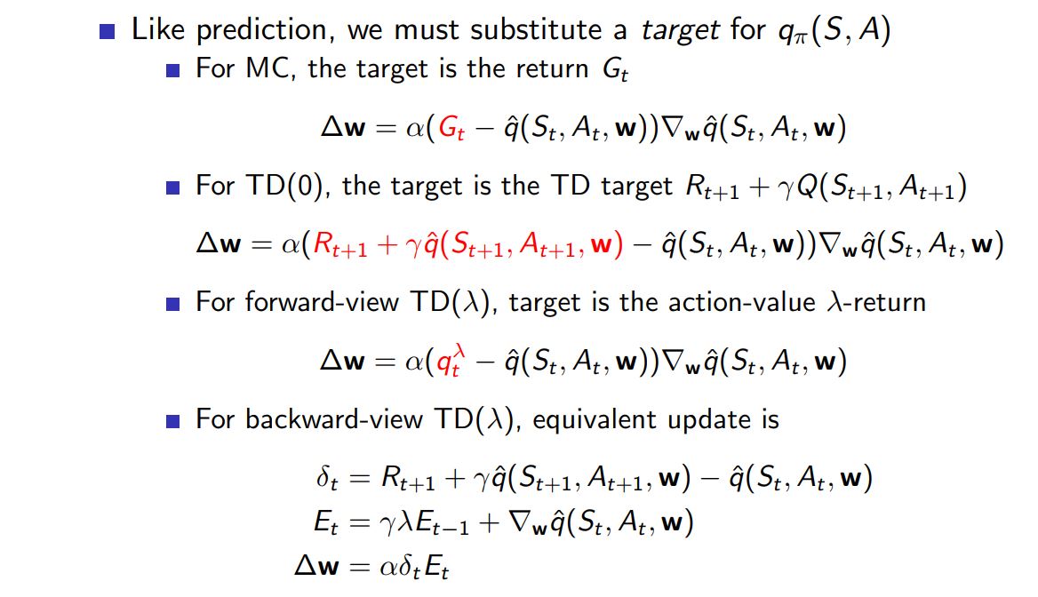
Incremental Control Algorithms 
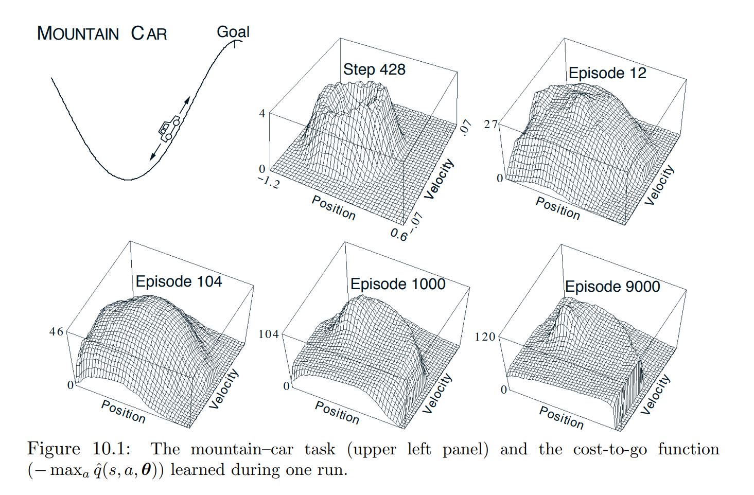
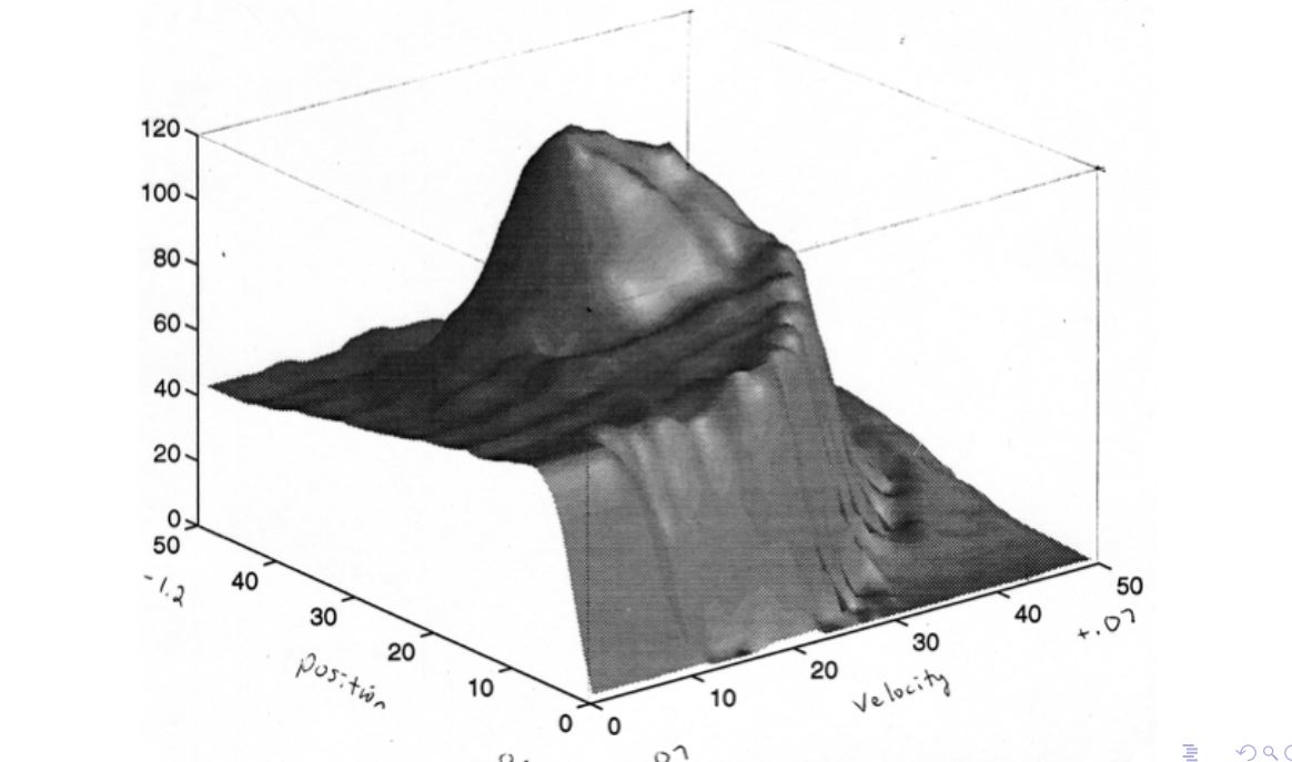
Mountain Car Problem
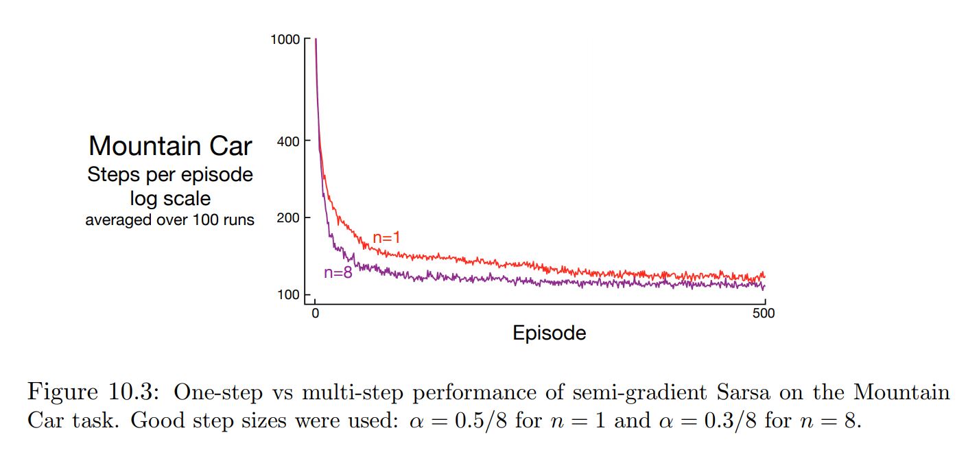
Single Step vs Multi Step
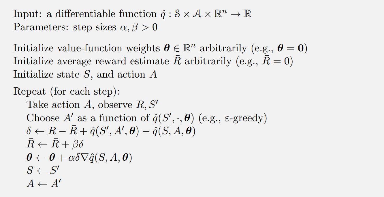
Episodic semi-gradient one-step Sarsa
- Target: ### $$ G_t = R_{t+1}+ \gamma \hat{q}(S_{t+1},A_{t+1},\theta _t)$$
- Gradient: ### $$ \theta_{t+1} = \theta_t + \alpha[ G_t -\hat{q}(S_t,A_t,\theta_t)] \nabla\hat{q}(S_t,A_t,\theta_t) $$
Episodic n-step Semi-gradient Sarsa
- Target: ### $$ G_t^{(n)} = R_{t+1}+\gamma R_{t+2} + ... + \gamma^{n-1}R(t+n) +\gamma^n \hat{q}(S_{t+n},A_{t+n},\theta _{t+n-1})$$
- Gradient: ### $$ \theta_{t+n} = \theta_{t+n-1} + \alpha[ G_t^{(n)} -\hat{q}(S_t,A_t,\theta_{t+n-1})] \nabla\hat{q}(S_t,A_t,\theta_{t+n-1}) $$
Single Step vs Multi Step
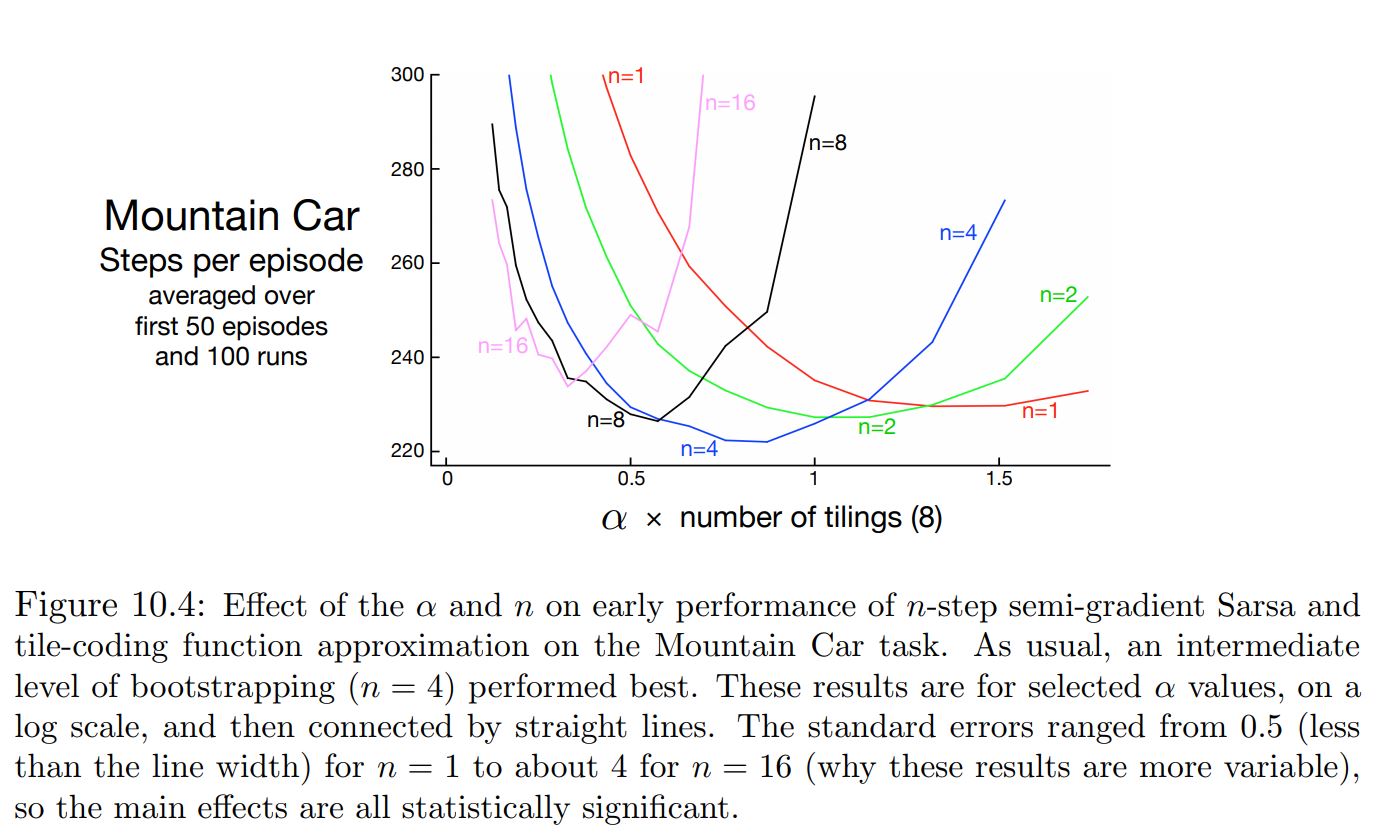
Effect of learning rate
Study of λ: Should We Bootstrap? 
Average Reward 
Average Reward
- Classical Settings:
- Discounting Setting
- Episodic Setting
- Average Reward
- applies to continuing problems
- there is no discounting
- Why?
- The discounted setting is problematic with function approximation,
- The average-reward setting is needed to replace it.
Average Reward
In average reward setting, the quality of a policy $\pi$ is defined as:
The average rate of rewards while following that policy, $\eta (\pi)$
### $$ \eta(\pi) = lim_{T \to \infty}\frac{1}{T} \sum_{t=1}^{T}{E[R_t|A_{0:t-1} \sim \pi]}$$ ### $$ \eta(\pi) = \sum_{s}{d_\pi(s) \sum_{a}{\pi(a|s) \sum_{s',r}{p(s,r'|s,a)r}}}$$$d_\pi$ is the steady-state distribution. ### $$ \sum_{s}{d_\pi(s) \sum_{a}{\pi(a|s,\theta) {p(s'|s,a)}}} = d_\pi(s')$$
Average Reward
In the average-reward setting, returns are defined in terms of differences between rewards and the average reward: ### $$G_t = R_{t+1} - \eta(\pi) + R_{t+2} - \eta(\pi) + ...$$
This is know as the differential return
- corresponding value functions are known as differential value functions.
Contrast with Discounted Value functions:
Differential value functions also have Bellman equations very similar to disconted value functions.
For disconted value functions
- For Average reward value Functions
Contrast with Discounted Value functions:
- For optimal disconted value functions
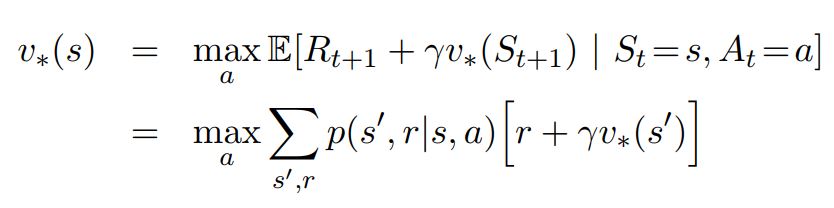
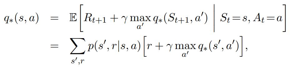
- For optimal Average reward value Functions
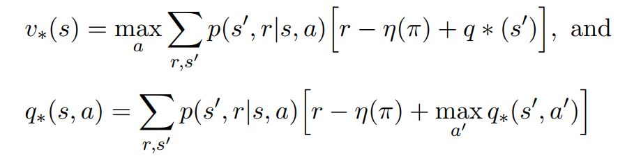
Contrast with Discounted Value functions:
There is also a differential form of the two TD errors:
For disconted value functions
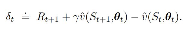
- For Average reward value Functions
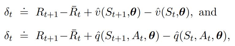
- $\bar{R}$ is an estimate of the average reward $\eta(\pi)$
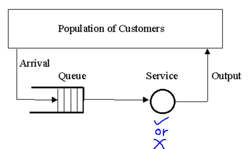
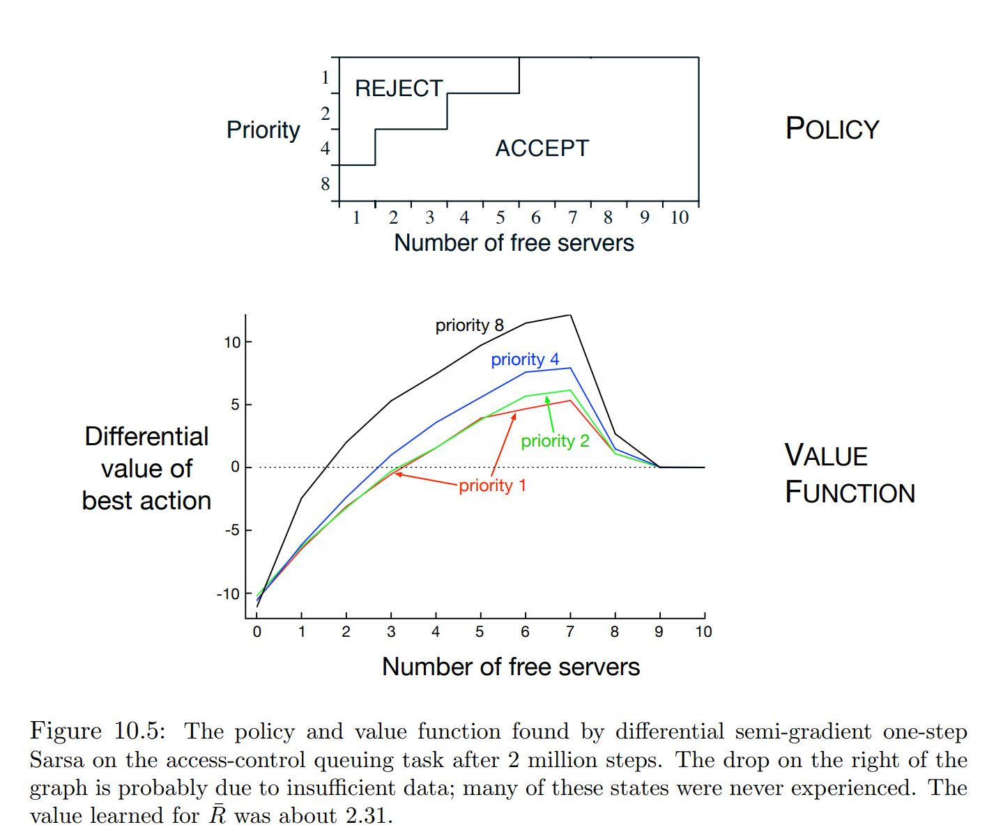
In each time step, the customer at the head of the queue is
- accepted (assigned to one of the servers) or
- rejected (removed from the queue, with a reward of zero).
On the next time step the next customer in the queue is considered.
The queue never empties
- the priorities of the customers are equally randomly distributed.
A customer can not be served if there is no free server;
Each busy server becomes free with probability p on each time step.
Task: Decide on each step whether to accept or reject the next customer,on the basis of
- His priority and
- The number of free servers,
So as to maximize long-term reward without discounting.
- average of the discounted returns is always $\eta(\pi)/(1 − \gamma)$
- The ordering of all policies in the average discounted return setting would be exactly the same as in the average-reward setting.
- The discounted case is still pertinent, or at least possible, for the episodic case.
Summary 
- To add