The Story So Far

An agent starts in a state s, takes an action a. The environment rewards the agent with reward r and computes the new state s’, the agent enters into. The way the agent chooses these actions, is called its policy. The goal of an agent is to accumulate as high rewards as it can. Hence, it boils down to figuring out an optimal policy that will result in a high cumulative reward.

We define a Q-function, i.e. Q(s,a) which determines how good a state and action pair (s,a) is. To define this quantitatively, we say what is the expected reward we might obtain when starting in state s, taking an action a and then following a policy $\pi$. There certainly exist policies that are optimal, meaning that they always select an action which is the best in the context. Let’s call the Q function for these optimal policies $Q^*$.

If we knew the true $Q^*$ function, the solution would be straightforward. We would just apply a greedy policy to it. That means that in each state s, we would just choose an action a that maximizes the function $Q^*$ – $argmax_a Q^*(s, a)$. Knowing this, our problem reduces to find a good estimate of the $Q^*$ function and apply the greedy policy to it.

Let’s write a formula for this function in a symbolic way. It is a sum of rewards we achieve after each action, but we will discount every member with $\gamma$: $Q^* (s, a) = r_0 + \gamma r_1 + \gamma^{2} r_2 + ...$ This can be recursively written as: $Q^* (s, a) = r_0 + \gamma Q^* (s', a)$

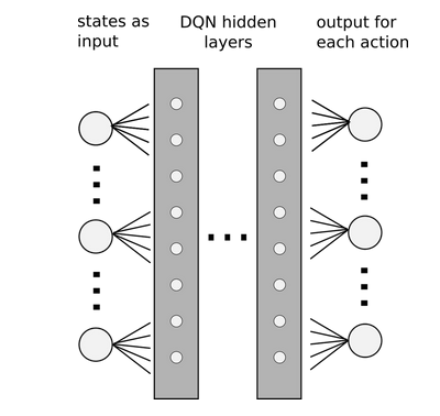
This might look good. But, real-world problems will have a infinite long state space where it will get difficult to store the values of all possible state-action pairs. So, we use neural networks to approximate these Q-values. This network will take the state as input and output the Q-values associated with all action values with that state. This network usually comprises of multiple hidden layers and is hence called a Deep Q-Network.

To stabilise this approximation of Q-values, ideas like Experience Replay and a separate Target Network were incorporated which resulted in success of DQNs.

What is the idea behind Experience Replay? During each simulation step, the agent perform an action a in state s, receives immediate reward r and come to a new state s’. Note that this pattern repeats often and it goes as (s, a, r, s’). The basic idea of online learning is that we use this sample to immediately learn from it.

We can use gradient descent on these accumulating ground truths and keep updating. But, the problem is the correlation in the incoming ground truths which often overfit and fail to generalise.

So, the idea behind experience replay is to store these transitions and at each time step, sample a random batch of transition and make an update.

What is the idea behind a separate Target Network? The target depends on the current network. A neural network works as a whole, and so each update to a point in the Q function also influences whole area around that point. And the points of Q(s, a) and Q(s’, a) are very close together, because each sample describes a transition from s to s’. This leads to a problem that with each update, the target is likely to shift. As a cat chasing its own tale, the network sets itself its targets and follows them. As you can imagine, this can lead to instabilities, oscillations or divergence.

To overcome this problem, researches proposed to use a separate target network for setting the targets. This network is a mere copy of the previous network, but frozen in time. After severals steps, the target network is updated, just by copying the weights from the current network. To be effective, the interval between updates has to be large enough to leave enough time for the original network to converge. Although, one of the disadvantages here is that this slows doen the learning process.

Other things that can be explored to complete the full chain: * Error Clipping * Double Q-Learning * Priortised Replay

Moving on: Building Concepts to Policy Gradients

Before getting deep into Policy Gradients, lets look at some of the concepts which will serve as buiding blocks. Firstly, agent’s actions are determined by a stochastic policy $\pi(s)$. Stochastic policy means that it does not output a single action, but a distribution of probabilities over actions, which sum to 1.0. We’ll also use a notation $\pi(a|s)$ which means the probability of taking action a in state s. Secondly, we define a value function $V(s)$ of policy $\pi$ as an expected discounted return, which can be viewed as a following recurrent definition: $V(s) = E_{\pi(s)}[ r + \gamma V(s') ]$ Basically, we weight-average the $r + \gamma V(s')$ for every possible action we can take in state s. Note again that there is no max, we are simply averaging. Action-value function $Q(s, a)$ is on the other hand defined plainly as: $Q(s, a) = r + \gamma V(s')$ simply because the action is given and there is only one following s’. Now, let’s define a new function $A(s, a)$ as: We call $A(s, a)$ an advantage function and it expresses how good it is to take an action a in a state s compared to average. If the action a is better than average, the advantage function is positive, if worse, it is negative. And lastly, let’s define $\rho$ as some distribution of states, saying what the probability of being in some state is. Consider the use two notations– $\rho^{s_0}$, which gives us a distribution of starting states in the environment and $\rho^\pi$, which gives us a distribution of states under policy $\pi$. In other words, it gives us probabilities of being in a state when following policy $\pi$.

Policy Gradients

Our neural network here, as opposed to DQN, with weights $\theta$ will now take an state s as an input and output an action probability distribution, $\pi_\theta$.

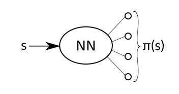
Given this action probability distribution, we can either sample or just choose the one with the highest probability. Eitherways, our aim is to make the policy better, i.e. optimize it. To do so, we first need some quality metric which discriminates a good policy from a bad policy. Consider a function $J(\pi)$ as a discounted reward that a policy $\pi$ can gain, averaged over all possible starting states $s_0$. $J(\pi) = E_{\rho^{s_0}}[V(s_0)]$ This does seem like a fair enough way to determine how good a policy is, but it’s hard to estimate. Good news is, that we don’t have to estimate this, we just need to improve it. That is, if we have the gradient of tis quantity, our mission is accomplished. Surprisingly, it turns out that there’s easily computable gradient of $J(\pi)$ function in the following form: $\nabla_\theta\;J(\pi) = E_{s\sim\rho^\pi,\;a\sim{\pi(s)}}[ A(s, a) \cdot \nabla_\theta\;log\;\pi(a|s) ]$ The proof for the same can be looked up in the slides.

The formula is quite intuitive. It informs us in what direction we have to change the weights of the neural network if we want the function $J(\pi)$ to improve. The second term inside the expectation, $\nabla_\theta\;log\;\pi(a\|s)$ , tells us a direction in which logged probability of taking action a in state s rises. Simply said, how to make this action in this context more probable. The first term, A(s, a), is a scalar value and tells us what’s the advantage of taking this action. Combined we see that likelihood of actions that are better than average is increased, and likelihood of actions worse than average is decreased. That sounds like a right thing to do.

One thing that remains to be explained is how we compute the A(s, a) term. $A(s, a) = Q(s, a) - V(s) = r + \gamma V(s') - V(s)$. It is sufficient to know the value function $V(s)$ to compute $A(s, a)$.

The value function can also be approximated by a neural network, just as we did with action-value function in DQN. Compared to that, it’s easier to learn, because there is only one value for each state.

Actor-Critic

We can use the same neural network for estimating $\pi(s)$ to estimate $V(s)$. The final architecture then looks like this:

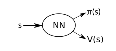
So we have two different concepts working together. The goal of the first one is to optimize the policy, so it performs better. This part is called actor. The second is trying to estimate the value function, to make it more precise. That is called critic.

Asynchronous Advantage Actor-Critic Agent (A3C)

We have already seen in detail the meaning of the two A’s and one C in A3C. What is remaining is the significance of ‘Asynchronous’. We saw that correlated samples in DQN caused a hinderance in the learning of a good Q-function. To overcome this, we used Experience Replay in DQN. But there’s another way to break this correlation while still using online learning. We can run several agents in parallel, each with its own copy of the environment, and use their samples as they arrive. Different agents will likely experience different states and transitions, thus avoiding the correlation. Another benefit is that this approach needs much less memory, because we don’t need to store the samples. This is how the agent learns Asynchronously.

References:

1. https://jaromiru.com/2016/09/27/lets-make-a-dqn-theory/
2. https://jaromiru.com/2017/02/16/lets-make-an-a3c-theory/
3. https://medium.com/emergent-future/simple-reinforcement-learning-with-tensorflow-part-8-asynchronous-actor-critic-agents-a3c-c88f72a5e9f2