Contents:
1) Introduction
2) Multi-arm Bandit Problems
3) Action Value Methods
4) Improving Exploration in Simple Bandit Problem
Introduction 
Reinforcement Learning: Uses information that evaluates the actions taken rather than instructs by giving correct actions(as in supervised Learning).
Non-Associative setting: Learning to act in just one situation.
- Environment is not dynamic.
- Very simplified setting.
- Full reinforcement learning is much more complex.
Example of Associative setting: Driving, amount of time spent reading in a day.
Example of Non-Associative setting: k-Arm Bandit Problem, Animals learning not to fear stuffed animals.
Goal
- Show how evaluative feedback differs from instructive feedback.
- Give an introduction on how to solve Reinforcement learning problems.
Multi-arm Bandit Problems 
k-Armed Bandit Problem:
- Every time step you have k different options, or actions.
- receive a numerical reward chosen from a stationary probability distribution based on the action.
- objective: maximize the expected total reward over some time period.

Each action has an expected/mean reward given that that action is selected given by $q_* (a) $.
$q_* (a) $ can be written as:
$$ \mathbf{ q_* (a) = E(R_t | A_t = a) } $$Notation
- $A_t$ = action selected at time step $t$
- $R_t$ = corresponding reward (at time step $t$)
- $q_* (a) $ = Value of an arbitrary action 'a' .
- $Q_t(a)$ = Estimated action value function.
If $\mathbf{q_* (a) }$ is known: we will select action 'a' with highest $\mathbf{q_* (a) }$.
But we do not have $\mathbf{q_* (a) }$.What can we do?
We can find a close estimate $\mathbf{Q_t (a) \approx q_* (a) }$.
- Should we accept our estimate and derive actions?
- Should we try to improve our estimate?
Exploring vs Exploiting
At any time step: select action with highest $\mathbf{Q_t (a)}$ ==> Exploiting.
At any time step: select action which does not have the highest $\mathbf{Q_t (a)}$ ==> Exploring.
Why explore?
- To reduce the uncertainity of $\mathbf{Q_t (a)}$ for all actions.
- Through exploration, you may find an action with greater $\mathbf{Q_t (a)}$.
- Exploitation is the right thing to do to maximize the expected reward in one step,
- but exploration may produce the greater total reward in the long run.
This is the k-armed bandit problem, where Exploration and exploitation has to be balanced.
Now, we will look at how to solve it.
Action-Value Method 
Action-Value Method
- Find an estimate $Q_t(a) \sim q_*(a)$ for each action.
Sample-Average method
Simplest way of estimating $Q_t(a)$, given $ Q_t (a) \approx q_* (a) = E(R_t | A_t = a)$
$$ Q_t (a) = \frac{\sum^{t-1}_{i=1}{R_i . 1_{A_i = a}}}{\sum^{t-1}_{i=1}{1_{A_i = a}}} $$If the denominator is zero, then we instead define $Q_t(a)$ as some default value, such as $Q_1(a) = 0$.
Now that we have the estimate $Q_t(a) \forall a \in A$, we need to select an action to take:
Greedy Action Selection Method
$$ A_t = {argmax}_a Q_t (a) $$$\epsilon$ - Greedy Method
- Behave greedily most of the time,
- But every once in a while, with small probability $\epsilon$,
- Select randomly from amongst all the actions ,
- With equal probability independently of the action-value estimates.
$\quad$ $\quad$ or
$\quad$ A = any random Action with probability $\epsilon$
Basically, the pseudo code for above algo is:
Initialize $Q_t(a) \quad \forall a \in A$,
At each time step:
$\quad$Select an action $A_t = a $ by greedy / $\epsilon$-greedy action selection
$\quad$Calculate new $Q_t$
Minor point: Incremental Implementation
Simple Bandit Algorithm with $\epsilon$-greedy method 
Initialize, for a =1 to k:
$\quad$ Q(a) = 0
$\quad$ N(a) = 0
Repeat Forever:
$\quad$ A = $argmax_a Q(a) \quad $ with probabiility $ 1-\epsilon $
$\quad$ $\quad$ or
$\quad$ A = any random Action $\quad$ with probability $\epsilon$
$\quad$ R = reward(A)
$\quad$ N(A) = N(A) +1
$\quad$ Q(A) = Q(A) + $\frac{1}{n}\big[ R_n - Q_n\big]$
Problem Formulation - The 10-armed testbed 
Problem Formulation - The 10-armed testbed
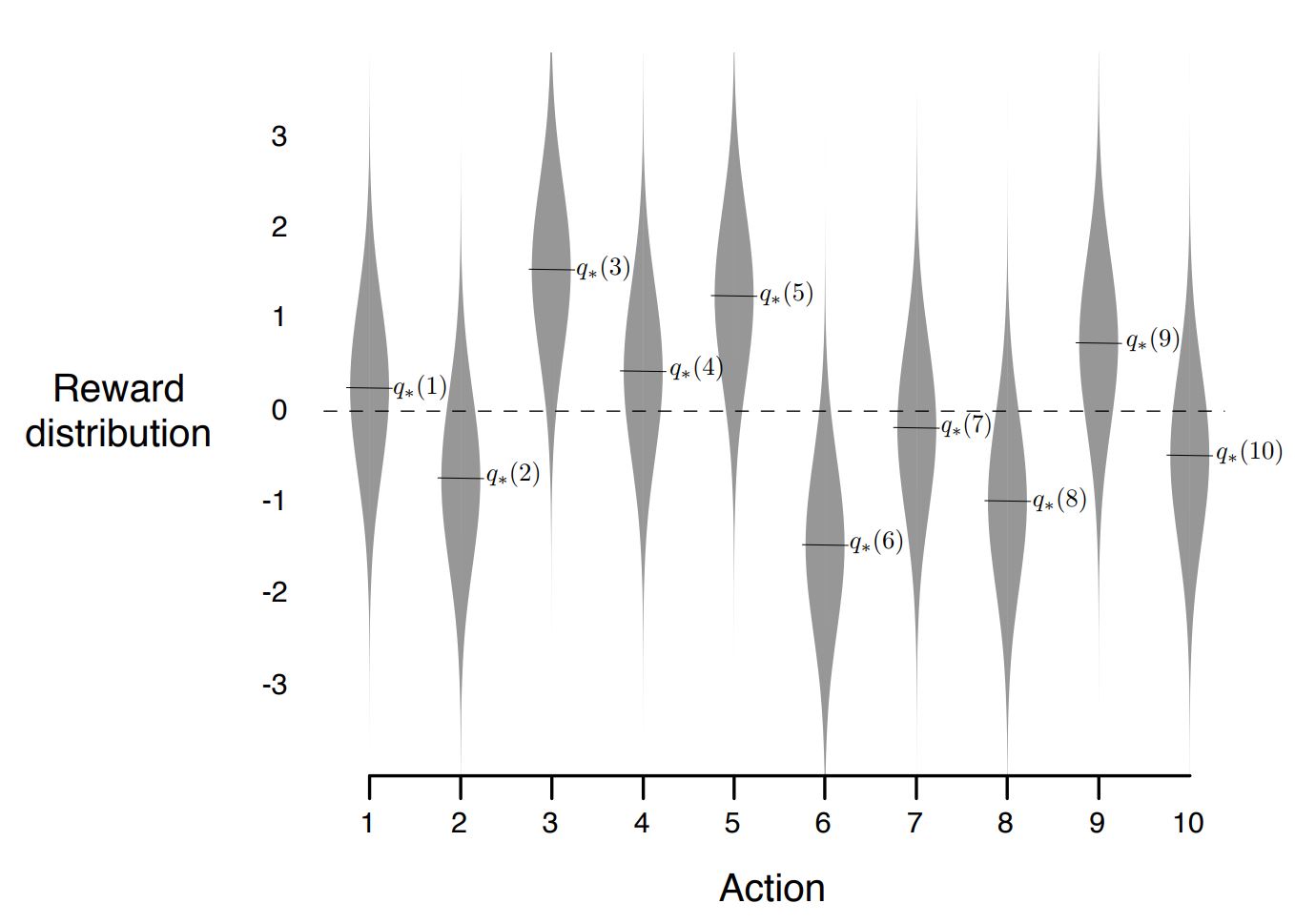
We randomly generated k-armed bandit problems with k = 10.
For each bandit problem,, the action values, $q_∗ (a)$, $a = 1, . . . , 10,$ were selected according to a normal (Gaussian) distribution with mean 0 and variance 1.
Then,when a learning method applied to that problem selected action $A_t$ at time $t$, the actual reward $R_t$ was selected from a normal distribution with mean $q_∗ (A_t)$ and variance 1.
- For any learning method, measure performance as it improves with experience over 1000 steps interaction.
- This is one run. Repeat this for 2000 independent runs.
- Obtain measures of the learning algorithm’s average behavior.
Results
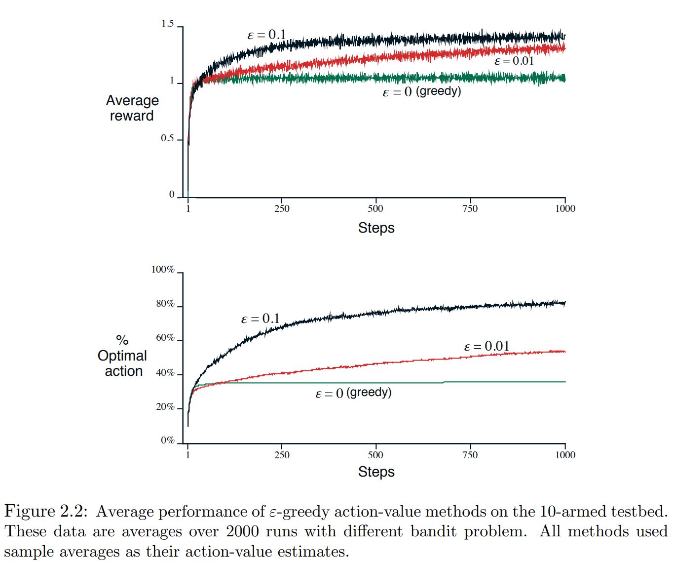
Question
When would $epsilon$-greedy method perform significantly better?
Update Rule of Simple Bandit Problem
In the pseudocode, given by:
This can be written as:
Tracking a Nonstationary Problem
Some problems are nonstationary, meaning reward function is not from a constant distribution.
In such cases, weight recent rewards more heavily than long-past ones.
This is done by:
This method is called: exponential, recency-weighted average.
Optimistic initial values
These methods are biased by their initial estimates.
Results
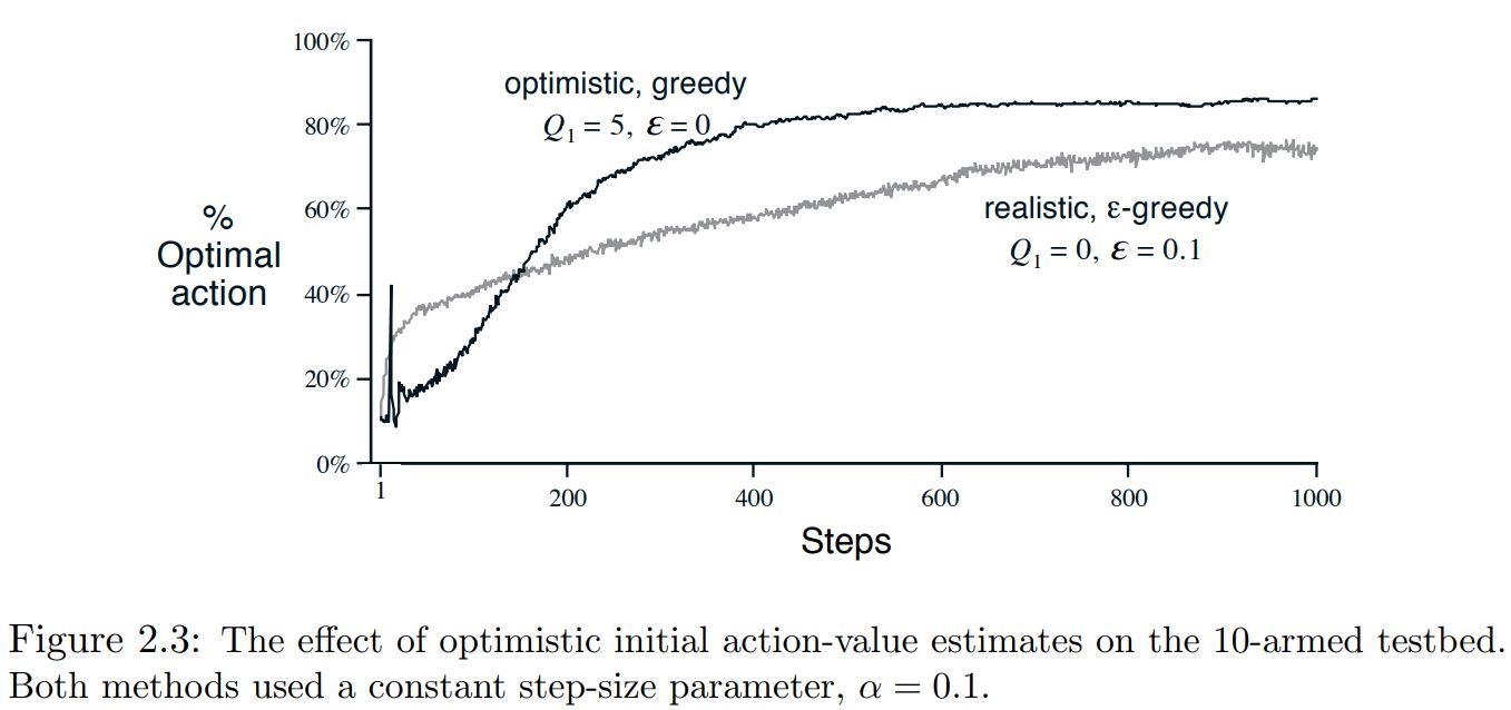
Optimistic initial values
- For the sample-average methods, the bias disappears once all actions have been selected at least once,
- methods with constant $\alpha$, the bias is permanent, though decreasing over time.
Initial action values can be used as a simple way of encouraging exploration.
However, this boost the exploration only once, in the start. It cannot be very useful in a non-stationary process.
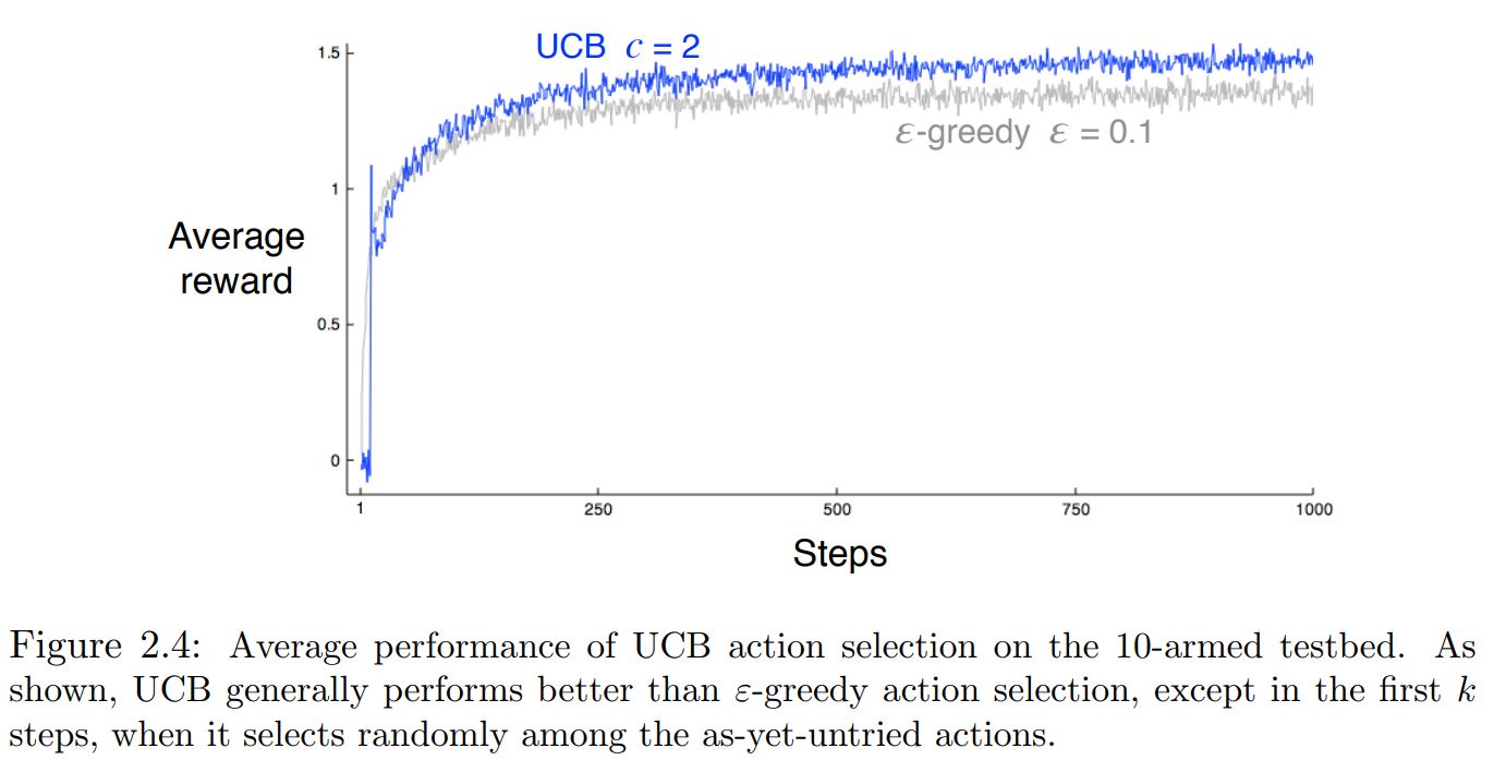
Upper-Confidence-Bound Action Selection
$$ A_t= argmax_a \bigg[ Q_t (a) + c \sqrt{\frac{log(t)}{N_t (a)}} \bigg] $$In upper confidence bound (UCB) action selection, the squareroot term is a measure of the uncertainty or variance in the estimate of $a$’s value.
Results
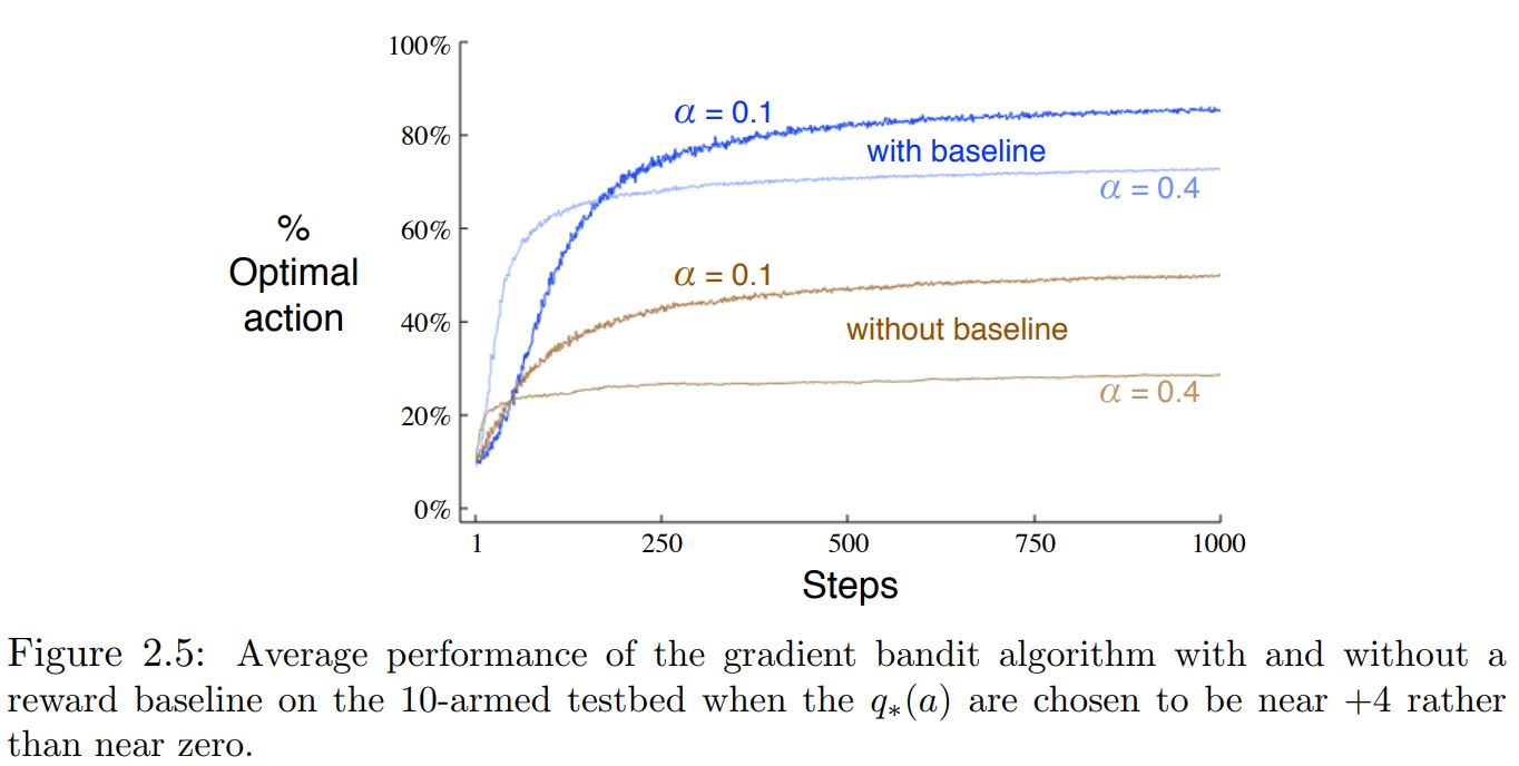
Gradient Bandit Algorithms
- Numerical preference $H_t (a)$ for each action $a$.
- The larger the preference, the more often that action is taken,
- Only the relative preference of one action over another is important;
Update Rules
$$ H_{t+1}(A_t) = H_t (A_t) + \alpha(R_t − \overline{R_{t}})(1− \pi_t (A_t)) $$and
$$ H_{t+1} (a) = H_t (a) - \alpha(R_t − \overline{R_{t}})\pi_t (a) \quad \forall a \neq A_t $$$\overline{R_{t}}$ is the average of all the rewards up through and including time t. It is also called the baseline reward.
Results
Summary 
- We have seen how Reinforcement learning is different from other forms of learning.
- We applied reinforcement learning to a very simple problem.
- We saw the importance of balancing exploration and exploitation
- The ε-greedy methods choose randomly a small fraction of the time,
- UCB methods choose deterministically but achieve exploration by subtly favoring at each step the actions that have so far received fewer samples.
- Gradient bandit algorithms estimate not action values, but action preferences, and favor the more preferred actions in a graded, probabilistic manner using a soft-max distribution.
- The simple expedient of initializing estimates optimistically causes even greedy methods to explore significantly.
Which is the best?
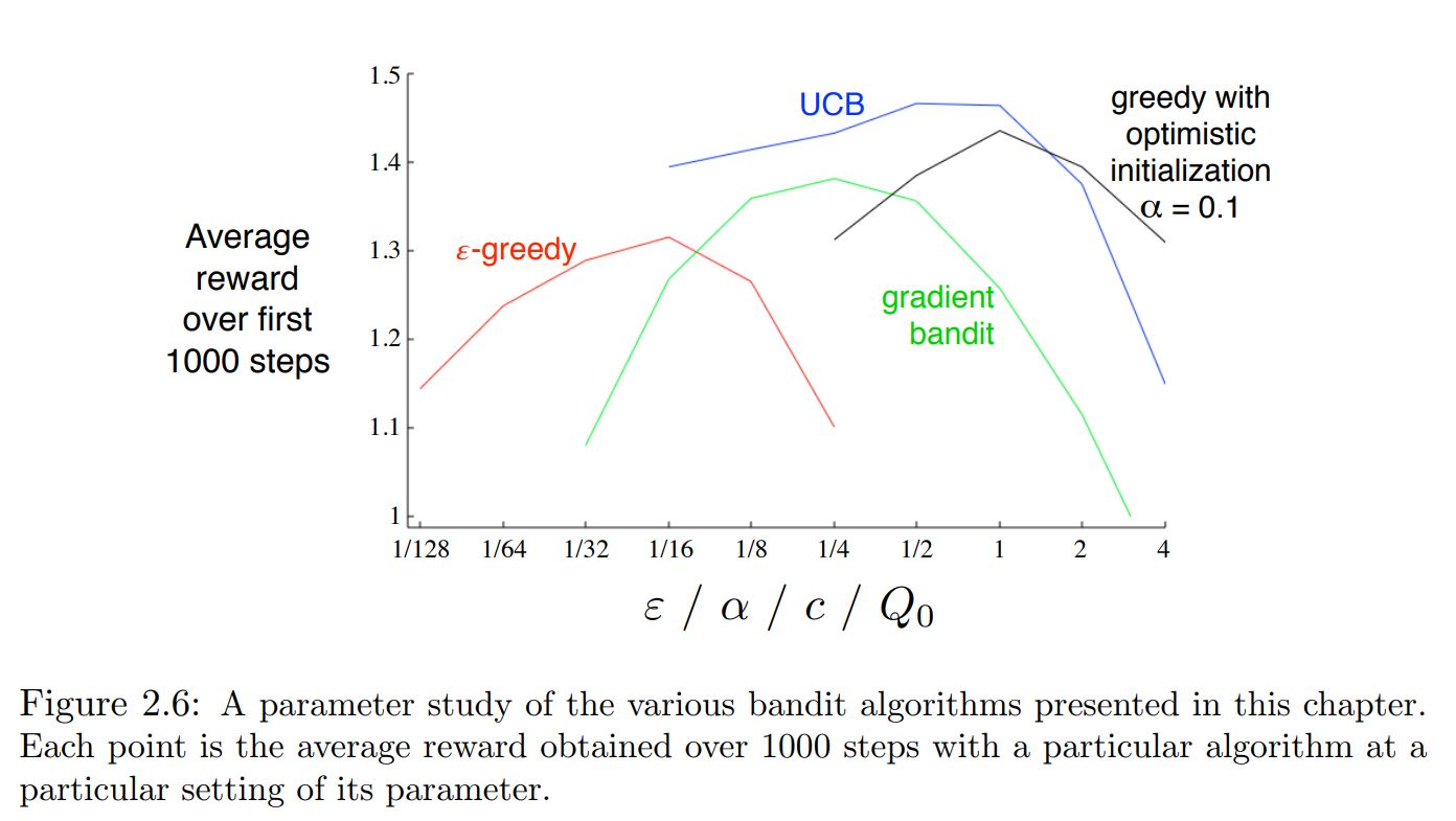
For the given problem, UCB performs the best.
No general statement should be made.
Different methods may perform better at different problems!