Temporal Difference Learning

Reference: Chapter 6, Sutton and Barto

Contents

• Introduction to Temporal Difference methods.

• Properties of Temporal Difference Methods

• One-step, tabular, modelfree TD methods
  • SARSA
  • Q-learning
  • Expected SARSA
  • Double Q- learning

Temporal Difference

• One of the central and most novel Ideas in Reinforcement learning.
• A one line Explaination is: In temporal Difference we improve Guesses towards Guesses before reaching terminal states.

Monte Carlo Methods

Roughly speaking, Monte Carlo methods wait until the return following the visit is known, then use that return as a target for $V(S_t)$.

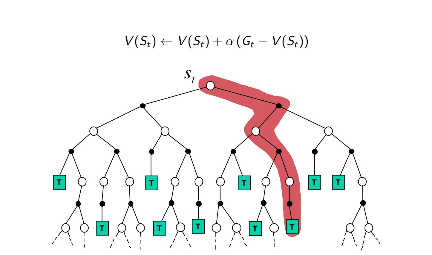
Constant $\alpha$ MC

$$ V(S_t) = V(S_t) + \alpha\big[ G_t - V(S_t) \big] $$

• $G_t$ is the actual return following time t,
• $\alpha$ is a constant step-size parameter.

Monte Carlo Backup

DP methods

Although DP methods update at every iteration, they use a model of the environment for the update. Basically they use, $p(s',r|s,a)$, the transition probability values.

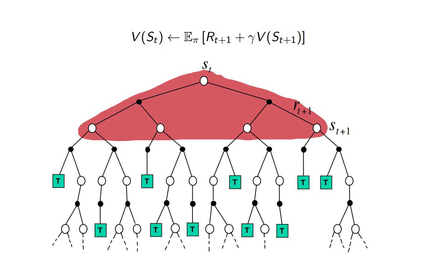
Iterative policy evaluation in DP

$$ V (s) = \sum_{a}\pi(a|s) \sum_{s',r}{p(s',r|s,a)\big[ r+\gamma V(s') \big]} $$

DP backup

Temporal Difference Prediction

TD methods need wait only until the next time step.

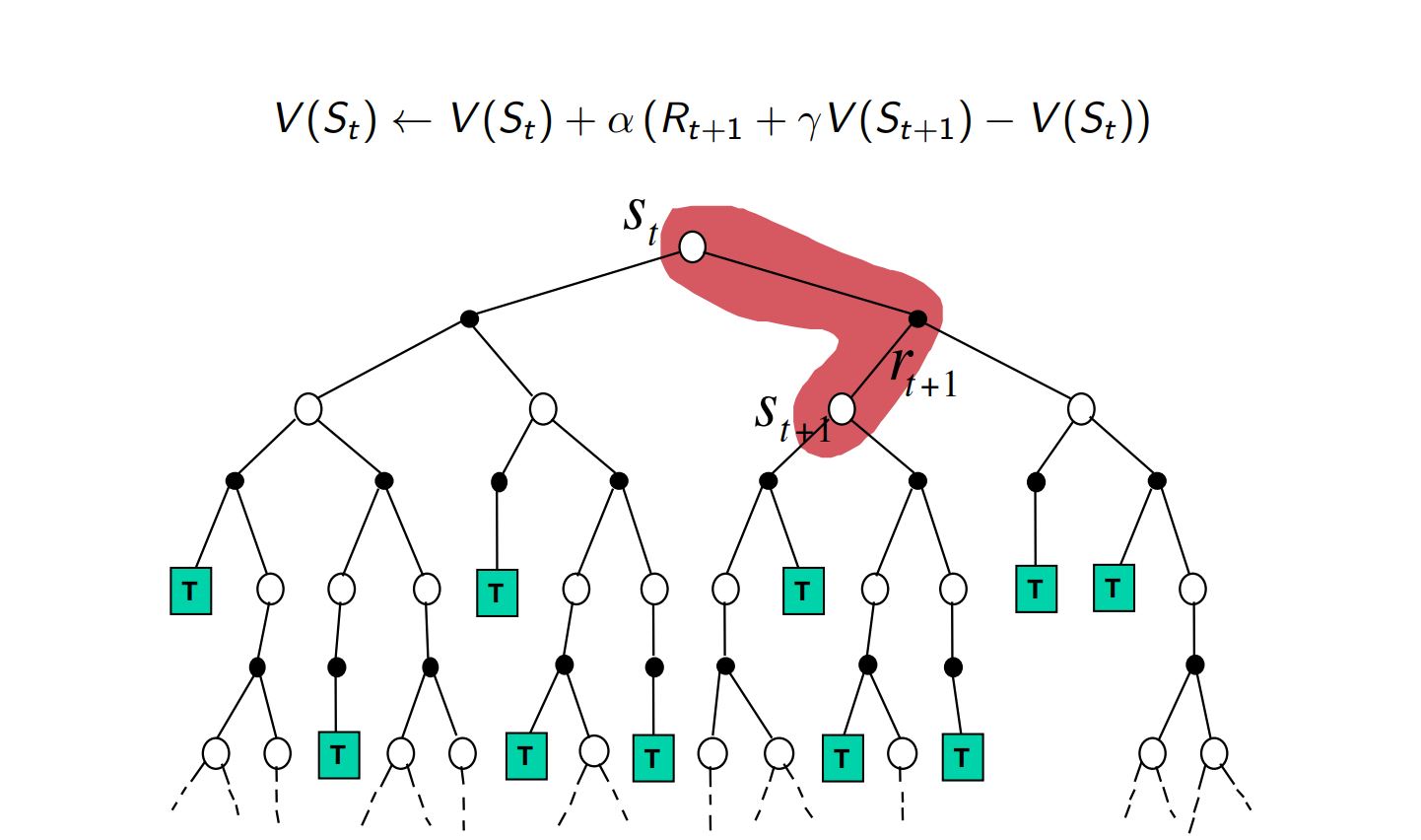
TD(0)

$$ V(S_t) = V(S_t) + \alpha\big[ R_{t+1} +\gamma V(S_{t+1})- V(S_t) \big] $$

• target for the Monte Carlo update is $G_t$, whereas the target for the TD update is $R_{t+1} + \gamma V(S_{t+1})$.
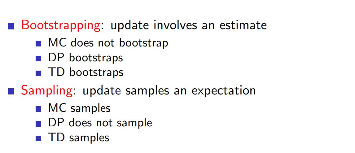
• Because the TD method bases its update in part on an existing estimate, we say that it is a bootstrapping method, like DP.

TD Backup

Monte Carlo Backup

DP backup

TD Backup

$ v_\pi (s) = E_\pi[G_t | S_t=s] = E_\pi[R_{t+1} + \gamma v_\pi(S_{t+1})| S_t = s]$

• Monte Carlo methods use an estimate of the first as a target,
• DP methods use an estimate of second as a target.

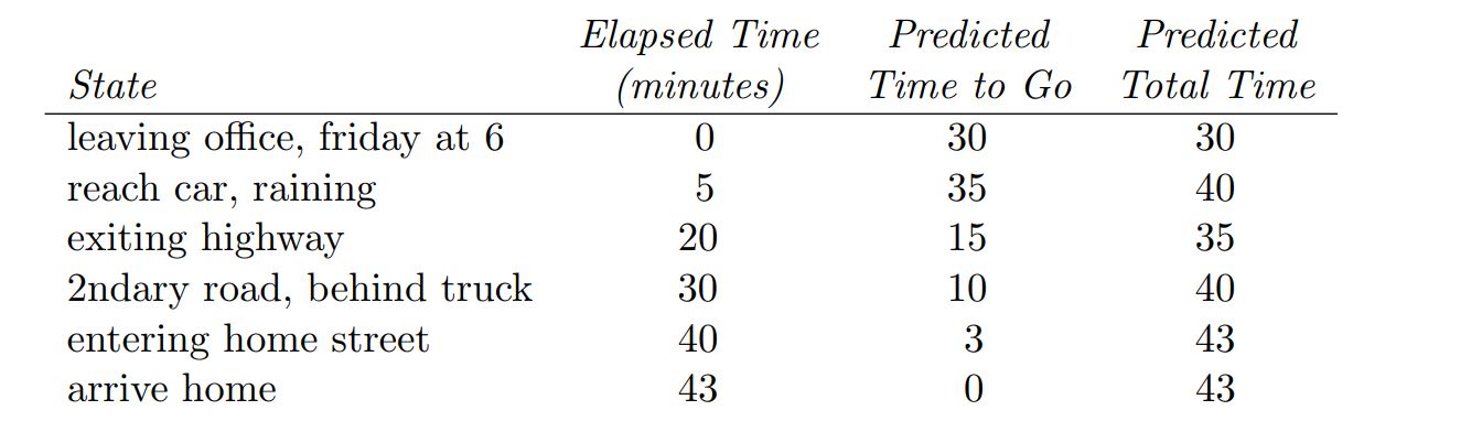
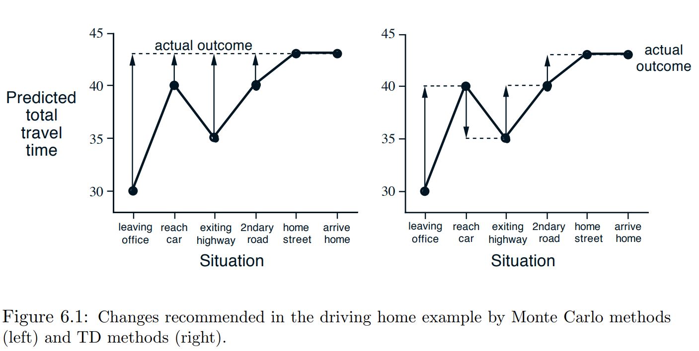
Example

Tabular TD for estimating $v_\pi$

Input: the policy $\pi$ to be evaluated
Initialize $V(s)$ arbitrarily (e.g., $V(s) = 0, \forall s \in S_+$)
Repeat (for each episode):
$\quad$Initialize $S$
$\quad$Repeat (for each step of episode):
$\quad$$\quad$ $A =$ action given by $\pi$ for $S$
$\quad$$\quad$Take action $A$, observe $R, S'$
$\quad$$\quad V (S) = V (S) + \alpha\big[R + \gamma V (S') − V (S)\big]$
$\quad$$\quad$S = S'
$\quad$until S is terminal

TD error

$ \delta_t = R_{t+1} + \gamma V (S_{t+1}) − V (S_t)$

Monte carlo error

$G_t - V(S_t) = \sum^{T-t-1}_{k=0}{\gamma^k \delta_{t+k}}$

Monte Carlo VS TD

Challenge:

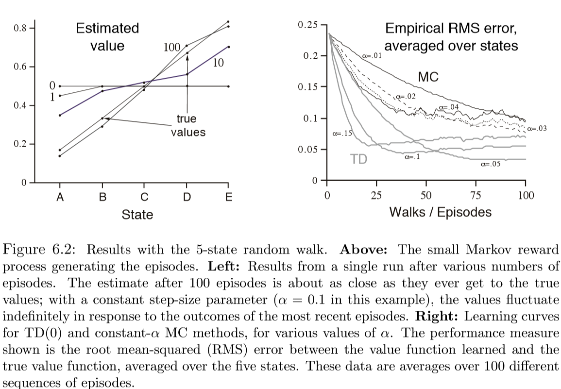
• A Markov Process with 5 states.
• Episodes sampled from a fixed behaviour policy (0.5 probability to transition to left or right)
• Theoretical Values of each state can be calculated(Using Probability)

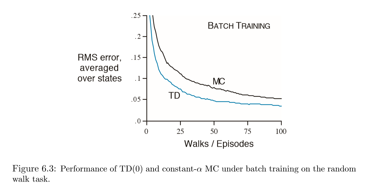
Results:

Properties of Temporal Difference Methods

Advantage of TD Methods

• Compared to DP methods, they do not require model of the environment, its rewards, and next state probability distribubtion.

• Compared to Monte Carlo methods, they are naturally implemented in an on-line, fully incremental fashion.

• Compared to Monte Carlo methods, TD can learn from incomplete sequences, can works in continuing (non-terminating) environments.

Some important points

• TD target $R_{t+1} + \gamma V(S_{t+1})$ is biased estimate of $v_\pi(S_t)$

• TD target has much lower variance than the MC target(returns $G_t$)

• For any fixed policy $\pi$, the TD algorithm has been proved to converge to $v_\pi$.

• Which method learns faster? Which makes the more efficient use of limited data? Not answered yet. Its an open question.

Batch Update

Suppose you have a fixed number of episodes,

• Given an approximate value function, V , we calculate the increments for every time step $t$ at which a non-terminal state is visited, but the value function is changed only once, by the sum of all the increments.

• Then all the available experience is processed again with the new value function to produce a new overall increment, and so on, until the value function converges.

• We call this batch updating because updates are made only after processing each complete batch of training data.

Batch-TD vs constant-$\alpha$ MC

Example

The following episodes are observed:

1) A, 0, B, 0
2) B, 1
3) B, 1
4) B, 1
5) B, 1
6) B, 1
7) B, 1
8) B, 0

Given this batch of data, what would you say are the optimal predictions, the best values for the estimates $V (A)$ and $V (B)$?

• Clearly, Optimal Value of B is the optimal value for $V (B)$ is $3/4$,

• But $V(A)$? Two reasonable answers:

• 100% of the times the process was in state A it traversed immediately to B. With no discounting, $V(A)=V(B)$.

• We have seen A once and the return that followed it was 0; we therefore estimate $V (A)$ as 0.

Now, which estimate does TD(0) make and which one does $\alpha-MC$ make?

If the process is seen as an instance of the following markov process:

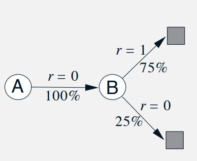
The First solution is right. This is the estimate that TD(0) makes.

If the process is Markov, we expect that the first answer will produce lower error on future data, even though the Monte Carlo answer is better on the existing data.

Batch Monte Carlo methods always find the estimates that minimize mean-squared error on the training set,

Whereas batch TD(0) always finds the estimates that would be exactly correct for the maximum-likelihood model of the Markov process.

Batch TD(0) converges to the certainty-equivalence estimate. Non-Batch methods can be understood as moving roughly in these directions.

One-step, tabular, modelfree TD methods

Sarsa: On-Policy TD Control

First, we estimate $q_\pi (s,a)$ instead of $v(s)$. The TD(0) equation for that would be

$$ Q(S_t, A_t) = Q(S_t, A_t) + \alpha \big[ R_{t+1} + \gamma Q(S_{t+1}, A_{t+1}) − Q(S_t, A_t) \big] $$

(update is done after every transition from a nonterminal state $S_t$).

This rule uses every element of the quintuple of events, $(S_t, A_t, R_{t+1}, S_{t+1}, A_{t+1})$, that make up a transition from one state–action pair to the next.

Hence this algorithm is named Sarsa.

Sarsa: An on-policy TD control algorithm

Initialize $Q(s, a), \forall s \in S, a \in A(s)$, arbitrarily, and $Q($terminal-state$, ·) = 0$
Repeat (for each episode):
$\quad$Initialize $S$
$\quad$Choose $A$ from $S$ using policy derived from $Q$ (e.g., $\epsilon$-greedy)
$\quad$Repeat (for each step of episode):
$\quad \quad$ Take action $A$, observe $R, S'$
$\quad \quad$ Choose $A'$ from $S'$ using policy derived from $Q$ (e.g., $\epsilon$-greedy)
$\quad \quad$ $Q(S, A) = Q(S, A) + \alpha \big[ R + \gamma Q(S', A') − Q(S, A) \big] $
$\quad \quad$ $S = S'; A = A';$
$\quad$ until $S$ is terminal

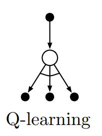
Q-learning: Off-Policy TD Control

As in value-iteration, we take the $Q(S', A')$, corresponding to the maximum from all possible action, instead of the actual action A' taken.

$$ Q(S_t, A_t) = Q(S_t, A_t) + \alpha \big[ R_{t+1} + \gamma {max}_a Q(S_{t+1}, a) − Q(S_t, A_t) \big] $$

The learned action-value function, $Q$, directly approximates $q∗$, the optimal action-value function, independent of the policy being followed.

Back up diagram

Q-learning: An off-policy TD control algorithm

Initialize $Q(s, a), \forall s \in S, a \in A(s)$, arbitrarily, and $Q($terminal-state$, ·) = 0$
Repeat (for each episode):
$\quad$Initialize $S$
$\quad$Repeat (for each step of episode):
$\quad \quad$ Choose $A$ from $S$ using policy derived from $Q$ (e.g., $\epsilon$-greedy)
$\quad \quad$ Take action $A$, observe $R, S'$
$\quad \quad$ $Q(S, A) = Q(S, A) + \alpha \big[ R +\gamma {max}_a Q(S', a) − Q(S, A) \big] $
$\quad \quad$ $S = S';$
$\quad$ until $S$ is terminal

Example : Cliff Walking

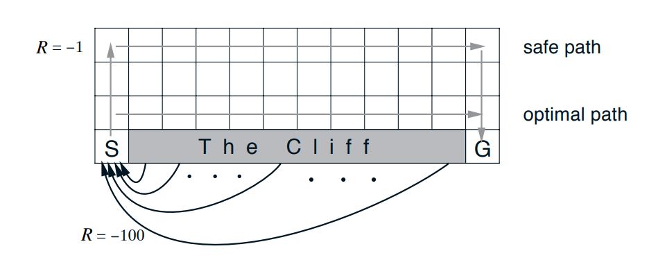
• A standard undiscounted, episodic task, with start and goal states,

• the usual actions causing movement up, down, right, and left.

• Reward is −1 on all transitions except those into the region marked “The Cliff.”

• Stepping into this region incurs a reward of −100 and sends the agent instantly back to the start.

Q-learning Vs Sarsa

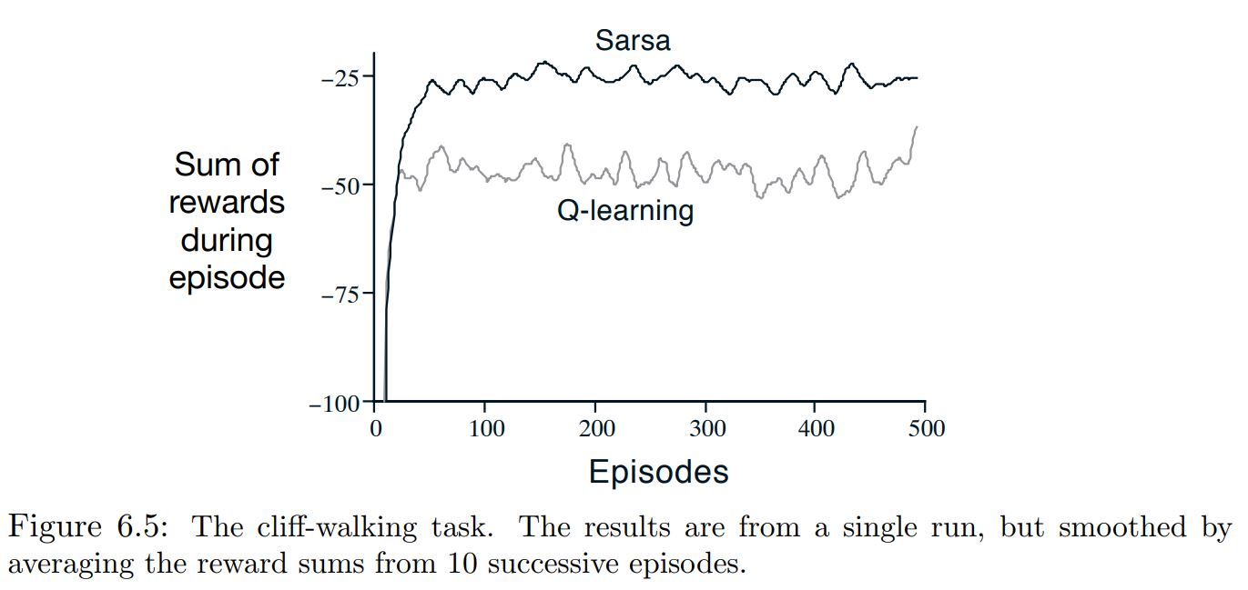
• Q-learning learns values for the optimal policy, that which travels right along the edge of the cliff.

• Unfortunately, this results in its occasionally falling off the cliff because of the $\epsilon$-greedy action selection.

• Sarsa, takes the action selection into account and learns the longer but safer path through the upper part of the grid.

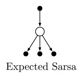
Expected Sarsa

Learning algorithm that is just like Q-learning except that instead of the maximum over next state–action pairs it uses the expected value, taking into account how likely each action is under the current policy.

$$ Q(S_t, A_t) = Q(S_t, A_t) + \alpha \big[ R_{t+1} + \gamma E(Q(S_{t+1}, A_{t+1}|S_{t+1}) − Q(S_t, A_t) \big] $$$$ Q(S_t, A_t) = Q(S_t, A_t) + \alpha \big[ R_{t+1} + \gamma \sum_{a}{\pi(a|S_t+1)Q(S_{t+1},a)} − Q(S_t, A_t) \big] $$

Back up diagram

Important Points

• Expected Sarsa is more complex computationally than Sarsa but, in return, it eliminates the variance due to the random selection of $A_{t+1}$.

• Expected Sarsa is stable on a wider range of step-size $\alpha$ than Sarsa.

• we can use a policy different from the target policy $\pi$ to generate behavior, in which case Expected Sarsa becomes an off-policy algorithm

• Expected Sarsa may completely dominate both of the other more-well-known TD control algorithms

Double Q Learning

Maximization Bias

• All the control algorithms that we have discussed so far involve maximization in the construction of their target policies.
• When maximum over estimated values is used implicitly as an estimate of the maximum value, it can lead to significant positive bias.

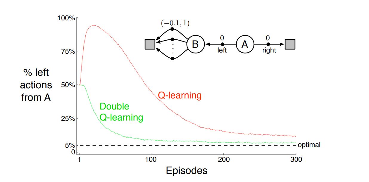
Example

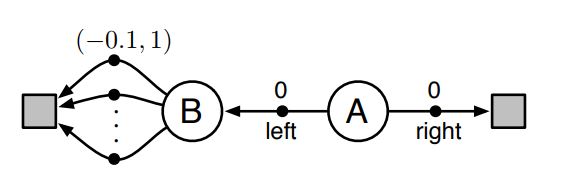
• The MDP has two non-terminal states A and B.
• Episodes always start in A with a choice between two actions, left and right.

• The right action transitions immediately to the terminal state with a reward and return of zero.
• The left action transitions to B, also with a reward of zero, from which there are many possible actions.

• All actions from B cause immediate termination with a reward drawn from a normal distribution with mean $−0.1$ and variance $1.0$.
• Thus, the expected return for any trajectory starting with left is $−0.1$, and thus taking left in state A is always a mistake.

• control methods may favor left because of maximization bias making B appear to have a positive value.

How to avoid maximing bias?

• Consider a bandit case in which we have noisy estimates of the value of each of many actions, obtained as sample averages of the rewards received on all the plays with each action.

• As we discussed above, there will be a positive maximization bias if we use the maximum of the estimates as an estimate of the maximum of the true values.

• One way to view the problem is that it is due to using the same samples (plays), both to determine the maximizing action and to estimate its value.

• Suppose we divided the plays in two sets and used them to learn two independent estimates, call them $Q_1(a)$ and $Q_2(a)$, each an estimate of the true value $q(a)$, for all $a \in A$.

• We could then use one estimate, say $Q_1$, to determine the maximizing action $A_∗ = argmax_a Q_1(a)$, and the other, $Q_2$, to provide the estimate of its value, $Q2(A_∗) = Q_2(argmax_a Q1(a))$.

• This estimate will then be unbiased in the sense that $E[Q_2(A_∗)] = q(A_∗)$.

• We can also repeat the process with the role of the two estimates reversed to yield a second unbiased estimate $Q_1(argmax_a Q_2(a))$.

Important Points

• Although we learn two estimates, only one estimate is updated on each play;
• Doubled learning doubles the memory requirements, but is no increase at all in the amount of computation per step.

Double Q-learning algorithm

Initialize $Q_1(s, a),Q_2(s, a), \forall s \in S, a \in A(s)$, arbitrarily, Initialize $Q_1($terminal-state$, ·) = Q_2($terminal-state$, ·) = 0$
Repeat (for each episode):
$\quad$Initialize $S$
$\quad$Repeat (for each step of episode):
$\quad \quad$ Choose $A$ from $S$ using policy derived from $Q_1$ and $Q_2$ (e.g., $\epsilon$-greedy in $Q_1+Q_2$)
$\quad \quad$ Take action $A$, observe $R, S'$
$\quad \quad$ With 0.5 probability:
$\quad \quad \quad Q_1(S, A) = Q_1(S, A) + \alpha \big[ R +\gamma Q_2(S',argmax_a Q_1(S',a)) − Q_1(S, A) \big] $
$\quad \quad$ Else:
$\quad \quad \quad Q_2(S, A) = Q_2(S, A) + \alpha \big[ R +\gamma Q_1(S',argmax_a Q_2(S',a)) − Q_2(S, A) \big] $
$\quad \quad$ $S = S';$
$\quad$ until $S$ is terminal

Double Q-learning vs Q-Learning