Planning and learning with tabular methods

Reference: Sutton and Barto Chapter 8

Contents

1) Introduction

2) Model Based RL

3) Dyna: Integrating Planning, Acting, and Learning

4) Prioritizing Sweeps

5) Planning as a part of action Selection(MCTS)

Introduction

• Model-Free RL
  • No model
  • Learn value function (and/or policy) from experience

• Model-Based RL
  • Learn a model from experience
  • Plan value function (and/or policy) from mode

In this Chapter we will learn how to learn a model directly from the environment and use planning to construct a value function/policy.

What is a model?

A model of the environment we mean anything that an agent can use to predict how the environment will respond to its actions.

Some models produce a description of all possibilities and their probabilities; these we call distribution models.

Other models produce just one of the possibilities, sampled according to the probabilities; these we call sample models.

What is planning?

We use the term Planning to refer to any computational process that takes a model as input and produces or improves a policy for interacting with the modeled environment.

state-space planning- Planning is viewed primarily as a search through the state space for an optimal policy or path to a goal.

plan-space planning- Planning is instead viewed as a search through the space of plans.Plan-space planning includes evolutionary methods and “partial-order planning".

In state space planning, two fundamental ideas:

1) All state-space planning methods involve computing value functions as a key intermediate step toward improving the policy, and

2) They compute their value functions by backup operations applied to simulated experience.

For eg: Dynamic Programming.

Difference between Planning and Learning:

The difference is that whereas planning uses simulated experience generated by a model, learning methods use real experience generated by the environment.

Model Based RL

• Advantages:
  • Can efficiently learn model by supervised learning methods
  • Can reason about model uncertainty

• Disadvantages:
  • First learn a model, then construct a value function
  • Two sources of approximation error

The model

• We will assume state space $S$ and action space $A$ are known.

• A model $M$ is a representation of an MDP $\{S, A,P, R\}$ parametrized by $\eta$.

• So a model $M = \{P_\eta,R_\eta\}$, where
  • $P_\eta \approx P$ represents state transitions
  • and $R_\eta \approx R$ represents the rewards.

• $$ S_{t+1} ~ P_\eta(S_{t+1} | S_t, A_t)$$ $$ R_{t+1} = R_\eta(R_{t+1} | S_t, A_t)$$

• Typically assume conditional independence between state transitions and rewards:
  $$ P [S_{t+1}, R_{t+1} | St , At ] = P [S_{t+1} | St, At] P [R_{t+1} | St , At] $$

Model Learning

Goal: estimate model $M_\eta$ from experience $\{S_1, A_1, R_2, ..., S_T \}$

• This is a supervised learning problem
  • $S_1, A_1 \rhd R_2, S_2$
    
  • $S_2, A_2 \rhd R_3, S_3$
    
  • .
    
  • .
    
  • .
    
  • $S_{T−1}, A_{T−1} \rhd R_T , S_T$

• Learning $s, a \rhd r$ is a regression problem,
• Learning $s, a \rhd s$ is a density estimation problem.

Pick loss function, e.g. mean-squared error, KL divergence, ...
Find parameters $\eta$ that minimise empirical loss

Examples of Models

• Table Lookup Model

• Linear Expectation Model

• Linear Gaussian Model

• Gaussian Process Model

• Deep Belief Network Mode

Table Lookup Model

• Model is an explicit MDP, $\hat{P}, \hat{R}$

• Count visits $N(s, a)$ to each state action pair

  • #### $$ \hat{P}^a_{s,s'} = \frac{1}{N(s, a)} \sum^{T}_{t=1}{\textbf{1}(S_t, A_t, St+1 = s, a,s')}$$

  • #### $$ \hat{R}^a_{s} = \frac{1}{N(s, a)} \sum^T_{t=1}{\textbf{1}(S_t , A_t = s, a)R_t} $$

• Alternatively,
  • At each time-step $t$, record experience tuple
    $\{S_t,A_t, R_{t+1}, S_{t+1}\}$
  • To sample model, randomly pick tuple matching $\{s,a,.,.\}$

Planning with a Model

• Given a model $M_\eta = \{P_\eta, R_\eta\}$

• Solve the MDP $\{S, A,P_\eta, R_\eta \}$

• Using favourite planning algorithm
  • Value iteration
  • Policy iteration
  • ...

Sample-Based Planning

• A simple but powerful approach to planning

• Use the model only to generate samples

• Sample experience from model $$ S_{t+1} ∼ P_\eta(S_{t+1} | S_t , A_t)$$ $$ R_{t+1} = R_\eta(R_{t+1} | S_t , A_t)$$

• Apply model-free RL to samples, e.g.:
  • Monte-Carlo control
  • Sarsa
  • Q-learning

• Sample-based planning methods are often more efficient

Disadvantages:

• We mostly have an imperfect model $\{P_\eta, R_\eta\} \approx \{P, R\}$

• Performance of model-based RL is limited to optimal policy for approximate MDP$\{S, A,P_\eta, R_\eta \}$

• i.e. Model-based RL is only as good as the estimated model When the model is inaccurate, planning process will compute a suboptimal policy.

• Solution 1: when model is wrong, use model-free RL
• Solution 2: reason explicitly about model uncertainty

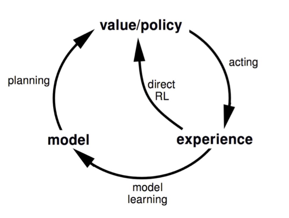
Dyna: Integrating Planning, Acting, and Learning

Real and Simulated Experience

• We consider two sources of experience
  • Real experience Sampled from environment (true MDP) $$ S' ~ P^a_{s,s'}$$ $$ R = R^a_s $$
  • Simulated experience Sampled from model (approximate MDP) $$ S' ~ P_\eta(S'|S,A) $$ $$ R' = R_\eta(S'|S,A) $$

• Real Experience has two roles:
  • Model Learning.
  • Direct Reinforcement learning.

Dyna

Tabular Dyna-Q Algorithm

Results

Results

When the model is wrong

• In previous section, the model started out empty, and was then filled only with exactly correct information.

• In general, Models may be incorrect because
  • The environment is stochastic.
  • Only a limited number of samples have been observed.
  • The model was learned using function approximation that has generalized imperfectly.
  • The environment has changed and its new behavior has not yet been observed.

Examples

Examples

Dyna +

• Agent keeps track for each state–action pair how many time steps elapsed since last tried in a real interaction.

• Greater the time elapsed, the greater (we might presume) the chance that the dynamics of this pair has changed and that the model of it is incorrect.

• To encourage behavior that tests long-untried actions,
  • a special “bonus reward” is given on simulated experiences involving these actions.
  • if the modeled reward $r$, and $\{S,A\}$ has not been tried in $\tau$ time steps,
    $r = r + κ\sqrt{\tau}$ , for some small κ.

Prioritized Sweeps

Introuction

• If simulated transitions are generated uniformly, then many wasteful backups will be made before stumbling onto one of these useful ones.

• In the much larger problems that are our real objective, the number of states is so large that an unfocused search would be extremely inefficient.

• In general, we want to work back from any state whose value has changed.

'Backward focusing' of planning computations

• the agent discovers a change in the environment and changes its estimated value of one state.

• The only useful one-step backups are those of actions that lead directly into the one state whose value has been changed.

• Hence we simulate those steps first.

• The frontier of useful backups propagates backward, it often grows rapidly.

• Hence we prioritize the backups according to a measure of their urgency.

• This is the idea behind prioritized sweeping.

Prioritized sweeping for a deterministic environment Algorithm

Results

Rod Maneuvering Task

• 14,400 possible states(36 angles, 20x20 Space)
• Actions: AlongRod,PerpRod,RotateL,RotateR
• Ackwardly placed immovable obstacles.

Planning as Part of Action Selection

Introduction

• The planning seen till now:
  • The gradual improvement of a policy/value function that is good in all states generally,
  • Not focused on any particular state.
  • Eg: Dyna, DP.

• A different outlook:
  • planning is begun and completed after encountering each new state $S_t$.
  • output is not really a policy,rather a single decision, the action $A_t$.
  • next step the planning begins anew with $S_{t+1}$ to produce $A_{t+1}$, and so on.

Some general Features of PPAS

• the values and policy are specific to the current state and its choices,
• They are typically discarded after being used to select the current action.
• useful in applications in which fast responses are not required.

Simulation-Based Search

• Forward search paradigm using sample-based planning
• Simulate episodes of experience from current time step with the model
• Apply model-free RL to simulated episodes

• Simulate episodes of experience from 'now' with the model ### $$ \{ s_t^k,A^k_t, R^k_{t+1},... S^k_T \} ^K_{k=1} \sim M_\nu $$

• Apply model-free RL to simulated episodes

  • Monte-Carlo control → Monte-Carlo search
  • Sarsa → TD search

Simple Monte Carlo Search

• With a perfect model and an imperfect action-value function, then deeper search will usually yield better policies.

Monte Carlo Tree Search

• One of the recent and successful developments in planning.
• Broken into two steps:
  • Evaluation
  • Simulation

Evaluation

Simulation

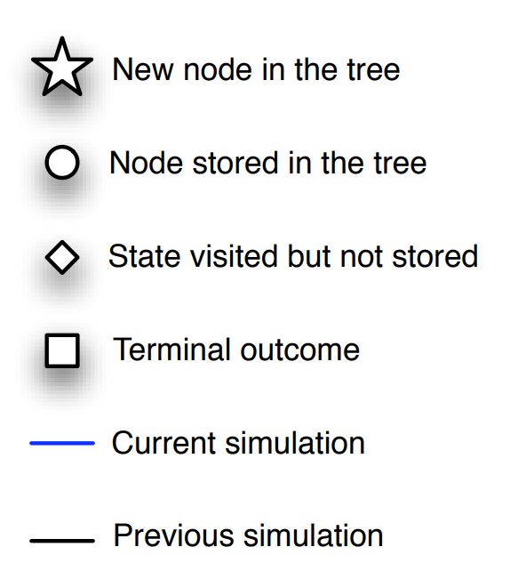
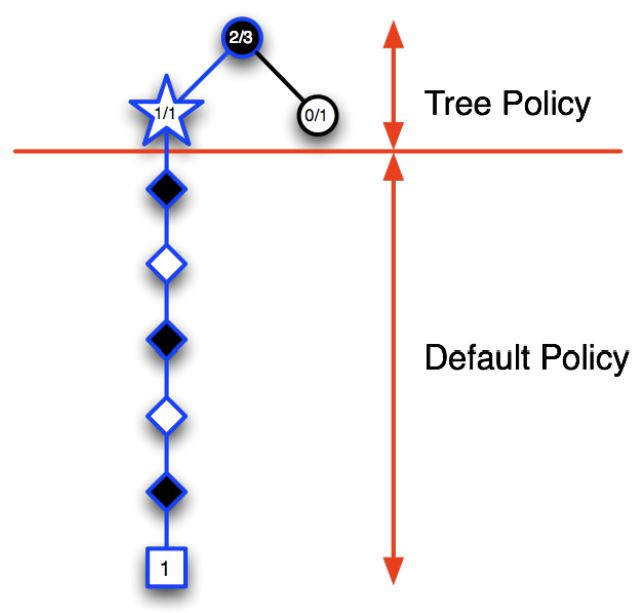
breakdown of MCTS

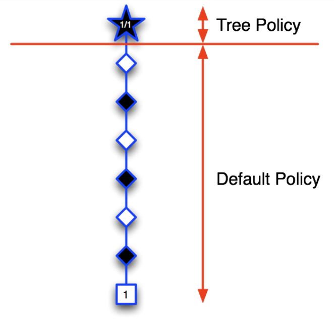
Steps:

1) Selection: A node in the current tree is selected by some informed means as the most promising node from which to explore further.

2) Expansion: The tree is expanded from the selected node by adding one or more nodes as its children.

• Each new child node is now a leaf node of the partial game tree, meaning
• None of its possible moves have been visited yet in constructing the tree.

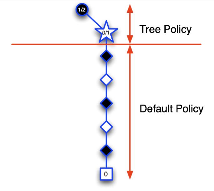
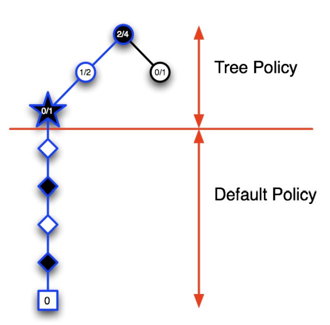
breakdown of MCTS

3) Simulation: From one of these leaf nodes, or another node having an unvisited move,a move is selected as the start of a simulation, or rollout, of a complete game.

• Moves are selected by a rollout policy.

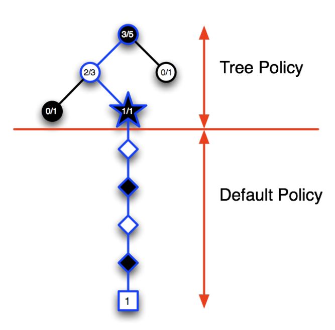
4) Backpropagation: The result of the simulated game is backed up to update statistics attached to the links in the partial game tree traversed.

Example

Advantages of MCTS

• Highly selective best-first search
• Evaluates states dynamically (unlike e.g. DP)
• Uses sampling to break curse of dimensionality
• Works for “black-box” models (only requires samples)
• Computationally efficient, anytime, parallelisable